关于stat的笔记

为stat230和stat231的部分复习.加上点(老人握拳.jpg)网课.

Descriptive Statistics

Data分为两种: Quantitative and Categorical.简单来说分为种类和数量 .

Quantitative data takes on numeric values that allow us to perform mathematical operations (like the number of dogs).
Categorical are used to label a group or set of items (like dog breeds - Collies, Labs, Poodles, etc.).

In categorical,可以分为有order和没有order的. Categorical Ordinal 和 Categorical Nominal .
In quantitative,分为 Continuous 和 Discrete .

Analyzing Quantitative Data

check:

Center
Mean平均数
Median中位数
Mode出现最多的数(可以有多个)
Spread(how spread out our data are from one another)
Range(max - min)
Interquartile Range(75% - 25%)
Standard Deviation(sometimes higher standard deviation means higher risk)
Variance
Shape
Outliers

注:
确定25%和75%:将数据分为1-50%和50-100%,再分别寻找中位数.
数据作为histagram时,重心往左靠是right-skewed(mean greater than median),往右是left-skewed.

aside: moving average

About outliers:
Understand why they exist. Reporting the 5 number summary values is often a better indication than measures like the mean and standard deviation when we have outliers.
Another word: 5 number summary works better with skewed data.
Normal distribution: work with standard deviation and mean.

Inferential Statistics

Using collected data to draw conclusions to a larger population.

Population - entire group of interest.
Parameter - numeric summary about a population
Sample - subset of the population
Statistic numeric summary about a sample

Example:

Population	Parameter	Sample	Statistic
10,000 students	proportion of all 10,000 students who drinks coffee	5000 students	73%

如果将每一组的数据做成distribution就是sampling distribution.

Sampling distribution

The sampling distribution is centered on the original parameter value.

The sampling distribution decreases its variance depending on the sample size used. Specifically, the variance of the sampling distribution is equal to the variance of the original data divided by the sample size used.
就是说在size较大的情况下,mean会接近原本的mean,但variance会跟sample size有关,公式:

variance is $\frac{\sigma^2}{n}$ .

例子:随机抽取array中的五个数并计算平均值.
(np是numpy)

1 2	sample1 = np.random.choice(students, 5, replace=True) sample1.mean()

重复多次获得histgram.这里获得的就是sampling distribution.
这里sample_props是空的,每次加进当次的mean,最后用sample来画图.

sample_props = []
for _ in range(10000):
    sample = np.random.choice(students, 5,replace=True)
    sample_props.append(sample.mean())

plt.hist(sample_props);

注意,此处的sample_props是list,为计算mean我们要将它转化成array.

1	sample_props = np.array(sample_props)

如果我们重复这个从抽取5变成抽取20,获得的hist更接近normal了.

Bootstrapping

Sampling with replacement.指选取某一个单位作为sample小组时,那个单位可以再被选取,也就是说sample小组可能拥有多个通一个单位的数据.
同样使用random.choice,with replace = True.

1	np.random.choice(die_vals, replace=True, size=20)

注:Bootstrapping assume sample is representative of the population.但是当sample large的时候,bootstrapping和tradition的method会接近.

Aside: (tradition confidence interval and hypothesis test)

T-test(link)
Two sample t-test(link)
Paired t-test(link)
Z-test(link)
Chi-squared test
F-test

Confidence interval

在不同的model中,confidence interval有不同的算法,具体参考sampling.

est \pm c*(s.e.)

z score calculator.

例子:
在数据里抽random sample.这里也可以用replace.

1 2	coffee_full = pd.read_csv('coffee.csv') coffee_red = coffee_full.sample(200)

再抽一次新的.

1	bootsamp = coffee_red.sample(200, replace = True)

依旧我们可以通过抽取来做sampling distribution.这里使用bootstrapping.

boot_means = []
for _ in range(10000):
    bootsamp = coffee_red.sample(200, replace = True)
    boot_mean = bootsamp[bootsamp['drinks_coffee'] == False]['height'].mean()
    boot_means.append(boot_mean)

plt.hist(boot_means); # Looks pretty normal

用percentile获得confidence interval.

1	np.percentile(boot_means, 2.5), np.percentile(boot_means, 97.5)

如果我们要比较喝咖啡的人和不喝咖啡的人是否有身高上的差距,我们可以对他们的身高做distribution.
如果他们的confidence interval不包括0,那么的确是有差距的.
如果要比较多个条件下的数据,我们可以使用query.

diffs_coff_under21 = []
for _ in range(10000):
    bootsamp = sample_data.sample(200, replace = True)
    under21_coff_mean = bootsamp.query("age == '<21' and drinks_coffee == True")['height'].mean()
    under21_nocoff_mean = bootsamp.query("age == '<21' and drinks_coffee == False")['height'].mean()
    diffs_coff_under21.append(under21_nocoff_mean - under21_coff_mean)

np.percentile(diffs_coff_under21, 2.5), np.percentile(diffs_coff_under21, 97.5)
# For the under21 group, we have evidence that the non-coffee drinkers are on average taller

我们还可以给两头的tail画线.

low, upper = np.percentile(diffs_coff_under21, 2.5), np.percentile(diffs_coff_under21, 97.5)
plt.hist(diffs_coff_under21);
plt.axvline(x=low, color='r', linewidth=2);
plt.axvline(x=upper, color='r', linewidth=2);

Aside: (term)
Margin of error is half the confidence interval width, and the value that you add and subtract from your sample estimate to achieve your confidence interval final results.

Simpson’s paradox

辛普森悖论(wiki),一个有名的分组讨论时会出错的悖论.

Bayer’s theorem

Bayer’s formula: $P(A \mid B)$ = ${P(B \mid A)P(A)}$ / ${P(B)}$ .

注: $P(A \mid B)$ is a conditional probability: the likelihood of event $A$ occurring given that $B$ is true.

其中 $P(A, B) = P(A \mid B) P(B)$ 也是A和B同时发生的概率.

Normal distribution

我觉得wiki说的挺好的,详细程度堪比cheatsheet,wiki.

Variable: mean $\mu$ , variance $\sigma^2$ .

Formula: $f(x)={\frac {1}{\sigma {\sqrt {2\pi }}}}e^{-{\frac {1}{2}}\left({\frac {x-\mu }{\sigma }}\right)^{2}}$ .

Aside: 在normal和sampling distribution中常用的:
Central limit theorem(wiki)
When independent random variables are added, their properly normalized sum tends toward a normal distribution (informally a bell curve) even if the original variables themselves are not normally distributed.

Law of Large Numbers(wiki)
According to the law, the average of the results obtained from a large number of trials should be close to the expected value and will tend to become closer to the expected value as more trials are performed.
也就是larger sample size,更靠近原本的mean.小的时候可能比原本的mean大也可能小.

等会儿得去复习一下的…
Maximum likelihood estimation(wiki)
Method of moments(wiki)
Bayes estimator(wiki)

Parameters

Parameter	Statistic	Description
$μ$	$\bar x$	mean of a dataset
$π$	$p$	mean of a dataset with only 0 and 1 values - a proportion
$μ_1 - μ_2$	$\bar x_1 - \bar x_2$	difference in means
$π_1 - π_2$	$p_1 - p_2$	difference in proportions
$β$	$b$	A regression coefficient - frequently used with subscripts
$σ$	$s$	standard deviation
$σ^2$	$s^2$	variance
$ρ$	$r$	correlation coefficient

Practical vs Statistic significance

Statistic significance: Evidence from hypothesis tests and confidence interval that H1 is true.

Practical(实用) significance: Takes into consideration other factors of your situation that might not be considered directly in the results of your hypothesis test or confidence interval. Constraints like space, time, or money are important in business decisions. However, they might not be accounted for directly in a statistical test.

Hypothesis testing

将问题分为两种可能,一种是null(H0),一种是alternative(H1),再用数据来证明H0或者rejectH0.
Aside: Hypothesis tests and confidence interval tells info about parameters not statistics.

H0 is true before you collect any data.
H0 usually states there is no effect or that two groups are equal.
H0 and H1 are competing, non-overlapping hypotheses.
H1 is what we would like to prove to be true.
H0 contains an equal sign of some kind - either =, $\leq≤$ , or $\geq≥$ .
H1 contains the opposition of the null - either $\neq≠$ , >>, or <<.

俗称用p value判定.

d = \frac{est - H_{0value}}{s.e.}

Example(我觉得有点有趣的…):
“Innocent until proven guilty” where H0 == Innocent and H1 == guilty.

Two types of error:

False positive(type 1, notation: alpha)
Deciding the alternative H1 is true, when actually H0 is true.
False negatives(type 2, notation: beta)
Deciding the null H0 is true, when actually H1 is true.

注意,如果(wlog)type 1 error会造成的损失比type 2大很多很多,我们应当调整alpha和beta的值.
eg: α = 0.01, β = 0.05.

用confidence interval测hypothesis testing我们还可以反向测.
使用numpy中的normal来判断H0的mean是否在我们得到的confidence interval中.

# 先通过sampling distribution获得means[] <- 有10000次循环的mean.

np.std(means)

# 70 is the mean of the distribution, also is our H0 assumption.
null_vals = np.random.normal(70, np.std(means), 10000)
plt.hist(null_vals);

# and compare to sample mean, see whether that fall into our histgram

当我们要做hypothesis testing的时候要考虑:

sample是否representative.
consider impact of sample size(large sample size -> statistically significant).

P-value

如果H0是true, the probability of observing your statistic (or one more extreme in favor of the alternative).
三种情况:

如果H0: μ <= 0, H1: μ > 0.
p-value是right end.
如果H0: μ => 0, H1: μ < 0.
p-value是left side.
如果H0: μ = 0, H1: μ ≠ 0.
p-value是两头.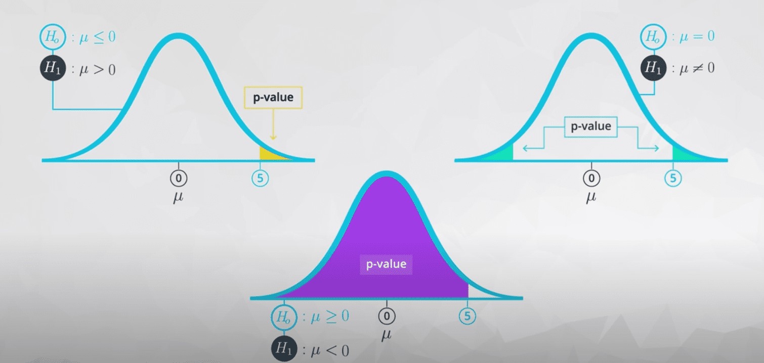

接着上头的代码.

null_vals = np.random.normal(70, np.std(means), 10000)

sample_mean = sample.height.mean()

(null_vals > sample_mean).mean() # 得到的是第一种P-value

# large p-value: should not move away from null hypotheses.
# 同理,小的p-value会reject H0.

如何定义大与小:compare to type I error.

pval ≤ α ⇒ Reject H0
pval > α ⇒ Fail to Reject H0

一个例子.

import numpy as np
import pandas as pd
import matplotlib.pyplot as plt
% matplotlib inline

np.random.seed(42)

df = pd.read_csv('classroom_actions.csv')
df.head()

# 比较实验组和样本组.

# get the average classroom time for control group
control_mean = df.query('group == "control"').total_days.mean()

# get the average classroom time for experiment group
experiment_mean = df.query('group == "experiment"').total_days.mean()

# display average classroom time for each group
control_mean, experiment_mean

# compute observed difference in classroom time
obs_diff = experiment_mean - control_mean

# display observed difference
obs_diff

# 用boostrapping找diffs的confidence interval

# create sampling distribution of difference in average classroom times
# with boostrapping
diffs = []
size = df.shape[0]
for _ in range(10000):
    b_samp = df.sample(size, replace=True)
    control_mean = b_samp.query('group == "control"').total_days.mean()
    experiment_mean = b_samp.query('group == "experiment"').total_days.mean()
    diffs.append(experiment_mean - control_mean)

# convert to numpy array
diffs = np.array(diffs)  

# plot sampling distribution
plt.hist(diffs);

# 我们这里的假设是新功能和旧功能没有(甚至更差)的假设,所以选的假定mean是0.

# simulate distribution under the null hypothesis
null_vals = np.random.normal(0, diffs.std(), diffs.size)  

# plot null distribution
plt.hist(null_vals)

# 比对diff

# plot line for observed statistic
plt.axvline(obs_diff, c='red')

# 算p-value
(null_vals > obs_diff).mean()

Bonferroni correction

在多次实验下校对tolerant error.

m = number of sets
α/m = new error

Other cerrection:

A/B testing

这个在旧博文写的更详细一些.

Null: 新的不比旧的好.
Alter: 新的好.

Novelty Effect: 新功能受到欢迎不是因为好,是因为新.

Regression

Machine Learning

Supervised(use input data to predict a value or label)
比如说用transaction的数据来预测fraud的行为.
Unsupervised(clustering data based on common characteristic)

作图的时候:

y轴为response variable(dependent,想要预测的值).
x轴为explanatory variable(independent,用来预测的值)

Term:

y

: 实际得到的数据.

\hat{y}

: 在预测线上的数据.

b0: intercept.
b1: slope.

Fitting a regression line:

Least squares algorithm

Find min $\sum_{i=1}^n (y_i - \hat{y_i})^2$ .

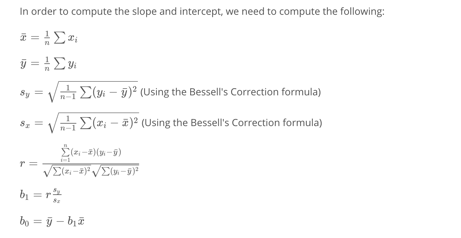
要使用这些公式我们可以用statsmodels.api里的function.

import statsmodels.api as sm
# 一定要有intercept
df['intercept'] = 1

lm = sm.OLS(df['price'], df[['intercept', 'area']])
results = lm.fit()
results.summary()

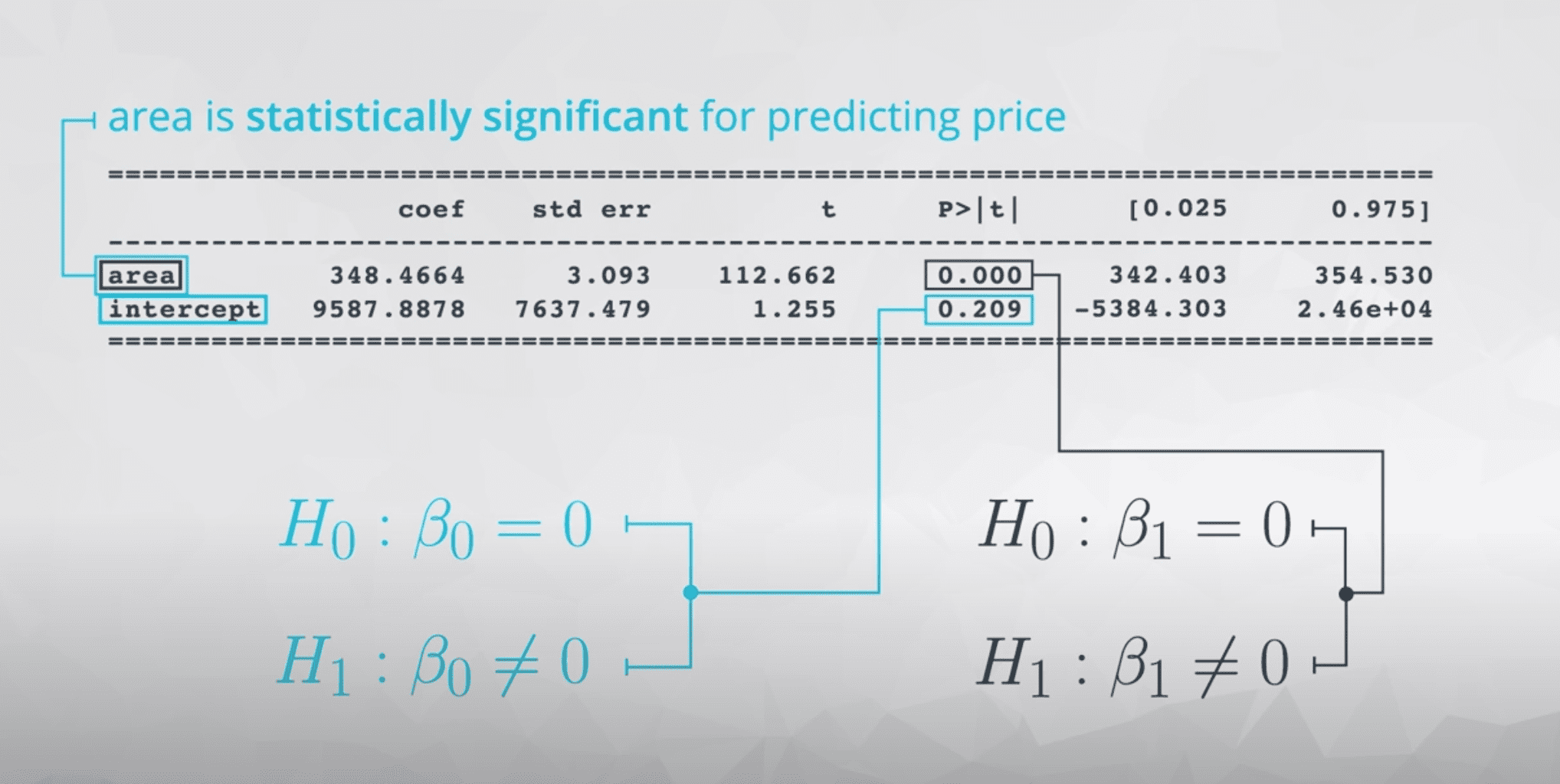
area coef is the slope we want(between area and price).

R-square: is the square of the correlation coefficient.
P-value: associated with each term in our model, is testing whether the population slope is equal to zero or not.

跟多个元素比较.
原理跟使用matrix, Find the optimal $\beta$ estimates by calculating $(X'X)^{-1}X'y$ ,一样.

df['intercept'] = 1

lm = sm.OLS(df['price'], df[['intercept', 'area', 'bathrooms', 'bedrooms']])
results = lm.fit()
results.summary()

如果我们要加入categorical 的parameter,我们使用dummy variable.
这个地方有点co250的技能了.
如果我们有ABC三种,那给3-1个dummy varibale.(因为x_A+x_B+x_C = 1,我们可以drop x_C)
We will need to drop one of the dummy columns in order to make your matrices full rank.
Drop掉的category就是跟保存的category数据做比较.

我们可以使用pandas里的get_dummies function.

import numpy as np
import pandas as pd
import statsmodels.api as sm;
import matplotlib.pyplot as plt
%matplotlib inline

df = pd.read_csv('./house_prices.csv')
df.head()

neighborhood_dummies = pd.get_dummies(df['neighborhood'])
df_new = df.join(neighborhood_dummies)
df_new.head()

# 注意这里我们drop了A
lm2 = sm.OLS(df_new['price'], df_new[['intercept', 'B', 'C']])
results2 = lm2.fit()
results2.summary()

# 我们除了P-value以外还可以通过看confidence interval的重合度来比较
plt.hist(df_new.query("C == 1")['price'], alpha = 0.3, label = 'C');
plt.hist(df_new.query("A == 1")['price'], alpha = 0.3, label = 'A');

plt.legend();

# 再加新的dummy直接加在后面就好…
type_dummies = pd.get_dummies(df['style'])
df_new = df_new.join(type_dummies)
df_new.head()

lm3 = sm.OLS(df_new['price'], df_new[['intercept', 'B', 'C', 'lodge', 'victorian', 'bedrooms', 'bathrooms']])
results3 = lm3.fit()
results3.summary()

当多组parameter有联系时(比如说area大的房子更可能有更多的bedroom和bathroom).

import seaborn as sb

# 查看三组paramter的关系
sb.pairplot(df[['area','bedrooms','bathrooms']]);

还可以查看VIF.
VIF的用法:每个系数的VIP是否超过10.如果有两个一起超过了10就说明这两个有很大的关联性,应当去掉一个作用不大的.

# price是我们的y, area + bedrooms + bathrooms是我们用的parameter
y, X = dmatrices('price ~ area + bedrooms + bathrooms', df, return_type = 'dataframe')

vif = pd.DataFrame()
vif["VIF Factor"] = [variance_inflation_factor(X.values, i) for i in range(X.shape[1])]
vif["features"] = X.columns

# show vif
vif

Scatter plot

plt.scatter(df['carats'], df['price']);
plt.xlabel('Carats');
plt.ylabel('Price');
plt.title('Price vs. Carats');

带预测线的plot.

## To show the line that was fit I used the following code from
## https://plot.ly/matplotlib/linear-fits/
## It isn't the greatest fit... but it isn't awful either


import plotly.plotly as py
import plotly.graph_objs as go

# MatPlotlib
import matplotlib.pyplot as plt
from matplotlib import pylab

# Scientific libraries
from numpy import arange,array,ones
from scipy import stats


xi = arange(0,100)
A = array([ xi, ones(100)])

# (Almost) linear sequence
y = df['MedianHomePrice']
x = df['CrimePerCapita']

# Generated linear fit
slope, intercept, r_value, p_value, std_err = stats.linregress(x,y)
line = slope*xi+intercept

plt.plot(x,y,'o', xi, line);
plt.xlabel('Crime/Capita');
plt.ylabel('Median Home Price');
pylab.title('Median Home Price vs. CrimePerCapita');

如果不是linear那可能是higher order term或者interaction term(x1 * x2).
注意,加入higher order term之后,the coefficients associated with area and area squared are not easily interpretable.
When adding interaction term:
The way that variable x1 is related to your response is dependent on value of x2.
我们用不同值的slope是否相同来判断,如果不同就得找interaction term.

Logistic Regression:将output局限在1与0之间,避免负数以及正无穷的outcome.

df['intercept'] = 1
log_mod = sm.Logit(df['fraud'], df[['intercept', 'weekday', 'duration']])
results = log_mod.fit()
results.summary2()

注意,因为是log_mod,我们要做一些转化.

np.exp(results.params)

1/_

df.groupby('prestige').mean()['admit']

关于summary2()

Confusion matrix

这个matrix还蛮好玩的.

	这一行写假设
这一行写实际	是A	是B
是A	只有看起来是A实际也是A才是预测正确了	横着看加起来是实际是A但有被看成其他的
是B	竖着加是看起来是A但有不是A但被看错了的

Recall: True Positive / (True Positive + False Negative). Out of all the items that are truly positive, how many were correctly classified as positive. Or simply, how many positive items were ‘recalled’ from the dataset.

Precision: True Positive / (True Positive + False Positive). Out of all the items labeled as positive, how many truly belong to the positive class.

Using confusion matrix by sklearn.
1&2

import numpy as np
import pandas as pd
from sklearn.linear_model import LogisticRegression
from sklearn.metrics import confusion_matrix, precision_score, recall_score, accuracy_score
from sklearn.model_selection import train_test_split
np.random.seed(42)

df = pd.read_csv('../data/admissions.csv')
df.head()

# get_dummies
df[['prest_1', 'prest_2', 'prest_3', 'prest_4']] = pd.get_dummies(df['prestige'])
X = df.drop(['admit', 'prestige', 'prest_1'] , axis=1)
y = df['admit']
X_train, X_test, y_train, y_test = train_test_split(X, y, test_size=0.20, random_state=0)

# confusion matrix
log_mod = LogisticRegression()
log_mod.fit(X_train, y_train)
preds = log_mod.predict(X_test)
confusion_matrix(y_test, preds)

precision_score(y_test, preds)
recall_score(y_test, preds)
accuracy_score(y_test, preds)

# graph
from ggplot import *
from sklearn.metrics import roc_curve, auc
%matplotlib inline

preds = log_mod.predict_proba(X_test)[:,1]
fpr, tpr, _ = roc_curve(y_test, preds)

df = pd.DataFrame(dict(fpr=fpr, tpr=tpr))
ggplot(df, aes(x='fpr', y='tpr')) +\
    geom_line() +\
    geom_abline(linetype='dashed')

一个stat有关的网站(web)

Aside: T-table

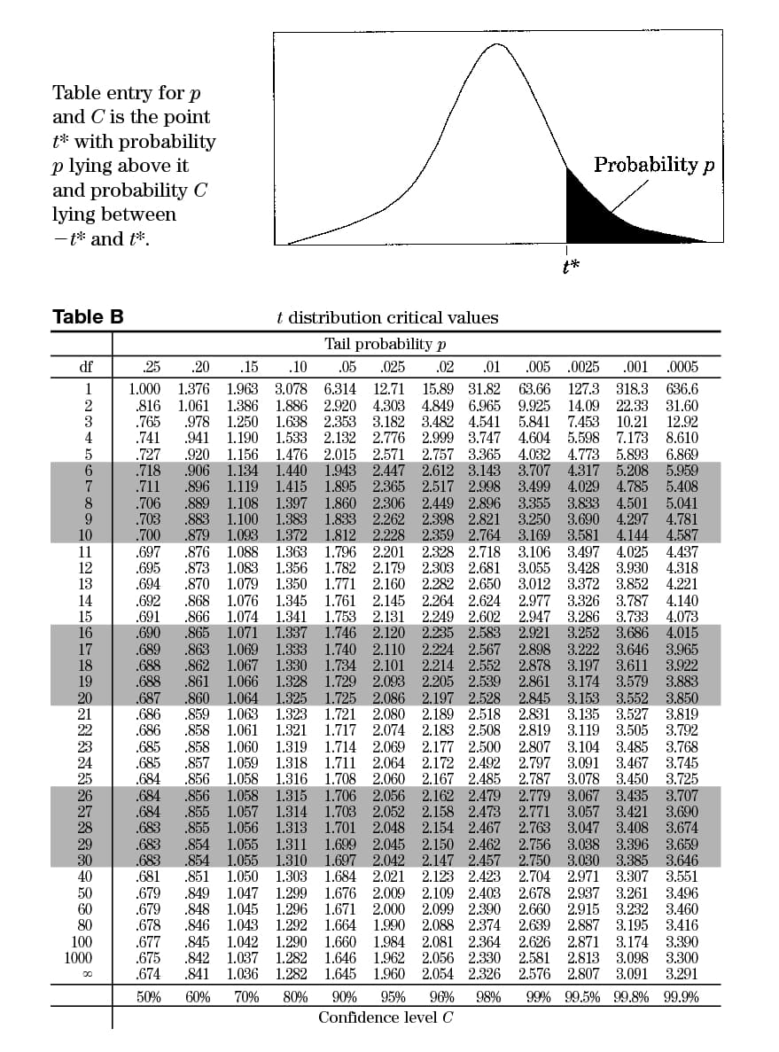
Z-table(link)

Aside: 因为data有时间相关(collected over time )的err,我们可以使用Durbin-Watson test.