为stat332的复习.附上没有过多关联的前情提要 .
332的精华在于推导每个model,再按需求套数据…所以整理的是各个model.
basic 基本判定方式有p-value与confidence interval.
CI :θ ~ ∼ N ( θ , V ( θ ~ ) ) \tilde{\theta} \sim N(\theta, V(\tilde{\theta})) θ ~ ∼ N ( θ , V ( θ ~ ) )
e s t ± c ∗ ( s . e . ) est \pm c*(s.e.) e s t ± c ∗ ( s . e . ) 等于θ ^ ± c ∗ V ( θ ~ ) \hat{\theta} \pm c* \sqrt{V(\tilde{\theta})} θ ^ ± c ∗ V ( θ ~ ) σ \sigma σ θ ^ ± c ∗ V ( θ ~ ) ^ \hat{\theta} \pm c* \sqrt{\hat{V(\tilde{\theta})}} θ ^ ± c ∗ V ( θ ~ ) ^ σ \sigma σ C ∼ N ( 0 , 1 ) C \sim N(0,1) C ∼ N ( 0 , 1 )
est指的是estimate的值.σ n \frac{\sigma}{\sqrt{n}} n σ
具体要参考model公式.
p-value :
d = e s t − H 0 v a l u e s . e . = θ ^ − θ 0 V ( θ ~ ) d = \frac{est - H_{0value}}{s.e.} = \frac{\hat{\theta} - \theta_0}{\sqrt{V(\tilde{\theta})}} d = s . e . e s t − H 0 v a l u e = V ( θ ~ ) θ ^ − θ 0 given estimator is θ ~ ∼ N ( θ , V ( θ ~ ) ) \tilde{\theta} \sim N(\theta, V(\tilde{\theta})) θ ~ ∼ N ( θ , V ( θ ~ ) ) D ∼ N ( 0 , 1 ) D \sim N(0,1) D ∼ N ( 0 , 1 ) σ \sigma σ D ∼ t n − 1 + c D \sim t_{n-1+c} D ∼ t n − 1 + c σ \sigma σ
H0指的是假设的值.
H 0 H_0 H 0 H a H_a H a P value
θ = θ 0 \theta = \theta_0 θ = θ 0 θ ≠ θ 0 \theta \neq \theta_0 θ = θ 0 2 P r ( D > a b s ( d ) ) 2Pr(D > abs(d)) 2 P r ( D > a b s ( d ) )
θ ≥ θ 0 \theta \geq \theta_0 θ ≥ θ 0 θ < θ 0 \theta < \theta_0 θ < θ 0 P r ( D < d ) Pr(D < d) P r ( D < d )
θ ≤ θ 0 \theta \leq \theta_0 θ ≤ θ 0 θ > θ 0 \theta > \theta_0 θ > θ 0 P r ( D > d ) Pr(D > d) P r ( D > d )
如果没有significance level默认:H 0 H_0 H 0 H 0 H_0 H 0 H 0 H_0 H 0 H 0 H_0 H 0
具体要参考model公式.
Side:两组数值时的variance(standard deviation的平方),aka pool variance,
s p 2 = ( n 1 − 1 ) s 1 2 + ( n 2 − 1 ) s 2 2 n 1 + n 2 − 2 s_p^2 = \frac{(n_1 - 1)s_1^2 + (n_2 - 1)s_2^2}{n_1+n_2-2} s p 2 = n 1 + n 2 − 2 ( n 1 − 1 ) s 1 2 + ( n 2 − 1 ) s 2 2 这里s 1 2 s_1^2 s 1 2 n 1 n_1 n 1 前情提要 的表格.
models Side:
Y j Y_j Y j μ \mu μ μ \mu μ π \pi π R j R_j R j μ \mu μ
Gauss’s theorem: Central limit theorem: Y 1 , . . . , Y n Y_1,...,Y_n Y 1 , . . . , Y n E ( Y i ) E(Y_i) E ( Y i ) μ \mu μ V ( Y i ) V(Y_i) V ( Y i ) σ 2 \sigma^2 σ 2 Y i Y_i Y i Y ˉ ∼ N ( μ , σ 2 n ) \bar{Y} \sim N(\mu, \frac{\sigma^2}{n}) Y ˉ ∼ N ( μ , n σ 2 )
Model1:
因为R j R_j R j Y i Y_i Y i
Y i = μ + R i Y_i = \mu + R_i Y i = μ + R i where R j ∼ N ( 0 , σ 2 ) R_{j} \sim N(0,\sigma^2) R j ∼ N ( 0 , σ 2 )
也可以写成Y i ∼ N ( μ , σ 2 ) Y_i \sim N(\mu , \sigma^2) Y i ∼ N ( μ , σ 2 )
with confidence interval: μ : y ˉ ± c ∗ S n \mu: \bar{y} \pm \frac{c*S}{\sqrt{n}} μ : y ˉ ± n c ∗ S n − 1 n - 1 n − 1
discrepancy: d = y ˉ − μ 0 s n d = \frac{\bar{y} - \mu_0}{\frac{s}{\sqrt{n}}} d = n s y ˉ − μ 0 D ∼ t n − 1 D \sim t_{n-1} D ∼ t n − 1
S = ∑ ( y i − y ˉ ) 2 n − 1 S = \sum \frac{(y_i - \bar{y})^2}{n - 1} S = ∑ n − 1 ( y i − y ˉ ) 2
___
Model2A:
Independent groups which have same variance.
Y i j Y_{ij} Y i j 是response of unit j in group i.
Y i j = μ i + R i j Y_{ij} = \mu_i + R_{ij} Y i j = μ i + R i j where R i j ∼ N ( 0 , σ 2 ) R_{ij} \sim N(0,\sigma^2) R i j ∼ N ( 0 , σ 2 )
with confidence interval: μ 1 : μ 1 ^ ± c ∗ S 1 n 1 \mu_1: \hat{\mu_1} \pm \frac{c*S_1}{\sqrt{n_1}} μ 1 : μ 1 ^ ± n 1 c ∗ S 1 n 1 − 1 n_1 - 1 n 1 − 1 OR μ 1 − μ 2 : μ 1 ^ − μ 2 ^ ± c ∗ σ ^ 1 n 1 + 1 n 2 \mu_1 - \mu_2: \hat{\mu_1} - \hat{\mu_2} \pm c*\hat{\sigma}\sqrt{\frac{1}{n_1} + \frac{1}{n_2}} μ 1 − μ 2 : μ 1 ^ − μ 2 ^ ± c ∗ σ ^ n 1 1 + n 2 1 n 1 + n 2 − 2 n_1 + n_2 - 2 n 1 + n 2 − 2
discrepancy: d = μ 1 ^ − μ 2 ^ − μ 0 σ ^ 1 n 1 + 1 n 2 d = \frac{\hat{\mu_1} - \hat{\mu_2} - \mu_0}{\hat{\sigma}\sqrt{\frac{1}{n_1} + \frac{1}{n_2}}} d = σ ^ n 1 1 + n 2 1 μ 1 ^ − μ 2 ^ − μ 0 D ∼ t n 1 + n 2 − 2 D \sim t_{n_1 + n_2 - 2} D ∼ t n 1 + n 2 − 2
___
Model2B:
Independent groups which have different variance.
Y i j Y_{ij} Y i j 是response of unit j in group i.
因为variance不一样,σ i 2 \sigma_i^2 σ i 2
Y i j = μ i + R i j Y_{ij} = \mu_i + R_{ij} Y i j = μ i + R i j where R i j ∼ N ( 0 , σ i 2 ) R_{ij} \sim N(0,\sigma_i^2) R i j ∼ N ( 0 , σ i 2 )
with confidence interval: μ 1 : μ 1 ^ ± c ∗ S 1 n 1 \mu_1: \hat{\mu_1} \pm \frac{c*S_1}{\sqrt{n_1}} μ 1 : μ 1 ^ ± n 1 c ∗ S 1 n 1 − 1 n_1 - 1 n 1 − 1 OR μ 1 − μ 2 : μ 1 ^ − μ 2 ^ ± c ∗ σ 1 2 ^ n 1 + σ 2 2 ^ n 2 \mu_1 - \mu_2: \hat{\mu_1} - \hat{\mu_2} \pm c*\sqrt{\frac{\hat{\sigma_1^2}}{n_1} + \frac{\hat{\sigma_2^2}}{n_2}} μ 1 − μ 2 : μ 1 ^ − μ 2 ^ ± c ∗ n 1 σ 1 2 ^ + n 2 σ 2 2 ^ n 1 + n 2 − 2 n_1 + n_2 - 2 n 1 + n 2 − 2
discrepancy: d = μ 1 ^ − μ 2 ^ − μ 0 σ 1 2 ^ n 1 + σ 2 2 ^ n 2 d = \frac{\hat{\mu_1} - \hat{\mu_2} - \mu_0}{\sqrt{\frac{\hat{\sigma_1^2}}{n_1} + \frac{\hat{\sigma_2^2}}{n_2}}} d = n 1 σ 1 2 ^ + n 2 σ 2 2 ^ μ 1 ^ − μ 2 ^ − μ 0 D ∼ t n 1 + n 2 − 2 D \sim t_{n_1 + n_2 - 2} D ∼ t n 1 + n 2 − 2
___
Model3:
model3测试的是一组两数据之间的difference(缩写为d).
Y d i = μ d + R d i Y_{di} = \mu_d + R_{di} Y d i = μ d + R d i where R d j ∼ N ( 0 , σ d 2 ) R_{dj} \sim N(0,\sigma_d^2) R d j ∼ N ( 0 , σ d 2 )
with confidence interval: μ d : y d ˉ ± c ∗ S d n d \mu_d: \bar{y_d} \pm \frac{c*S_d}{\sqrt{n_d}} μ d : y d ˉ ± n d c ∗ S d n d − 1 n_d - 1 n d − 1
discrepancy: d = μ d ˉ − μ 0 σ d ^ n d d = \frac{\bar{\mu_d} - \mu_0}{\frac{\hat{\sigma_d}}{\sqrt{n_d}}} d = n d σ d ^ μ d ˉ − μ 0 D ∼ t n d − 1 D \sim t_{n_d-1} D ∼ t n d − 1
___
Model4:
where we have n outcome, and each outcome is binary.
Y n ∼ N ( π , π ( 1 − π ) n ) \frac{Y}{n} \sim N(\pi,\frac{\pi(1-\pi)}{n}) n Y ∼ N ( π , n π ( 1 − π ) ) with confidence interval: π : π ^ ± c ∗ π ^ ( 1 − π ^ ) n \pi: \hat{\pi} \pm c*\sqrt{\frac{\hat{\pi}(1-\hat{\pi})}{n}} π : π ^ ± c ∗ n π ^ ( 1 − π ^ ) C ∼ N ( 0 , 1 ) C \sim N(0,1) C ∼ N ( 0 , 1 )
discrepancy: d = π ^ − π 0 π 0 ^ ( 1 − π 0 ^ ) n d = \frac{\hat{\pi} - \pi_0}{\sqrt{\frac{\hat{\pi_0}(1-\hat{\pi_0})}{n}}} d = n π 0 ^ ( 1 − π 0 ^ ) π ^ − π 0 C ∼ N ( 0 , 1 ) C \sim N(0,1) C ∼ N ( 0 , 1 )
Side:
y 1 , . . . , y n y_1,...,y_n y 1 , . . . , y n Y 1 , . . . , Y n Y_1,...,Y_n Y 1 , . . . , Y n Statistic is a function of the sample data, θ ^ \hat{\theta} θ ^ θ ^ \hat{\theta} θ ^ 我们可以把θ ^ \hat{\theta} θ ^ θ ~ \tilde{\theta} θ ~ θ ~ \tilde{\theta} θ ~
从θ ^ \hat{\theta} θ ^ θ ~ \tilde{\theta} θ ~ y 1 , . . . , y n y_1,...,y_n y 1 , . . . , y n Y 1 , . . . , Y n Y_1,...,Y_n Y 1 , . . . , Y n μ 1 ^ \hat{\mu_1} μ 1 ^ y 1 + ˉ \bar{y_{1+}} y 1 + ˉ μ 1 ~ \tilde{\mu_1} μ 1 ~ Y 1 + ˉ \bar{Y_{1+}} Y 1 + ˉ
___
Model5:
completely randomized design.
Y i j = μ i + τ i + R i j Y_{ij} = \mu_i + \tau_i + R_{ij} Y i j = μ i + τ i + R i j where R i j ∼ N ( 0 , σ 2 ) R_{ij} \sim N(0,\sigma^2) R i j ∼ N ( 0 , σ 2 ) i = 1 , 2 , . . . , t i = 1,2,...,t i = 1 , 2 , . . . , t j = 1 , 2 , . . . , r j = 1,2,...,r j = 1 , 2 , . . . , r
the # of units are i*j.μ \mu μ μ + τ i \mu + \tau_i μ + τ i τ i \tau_i τ i
R i j R_{ij} R i j is the distribution of values about the deterministic part of the model.
Constraints: τ 1 + τ 2 . . . + τ t = 0 \tau_1 + \tau_2 ... + \tau_t = 0 τ 1 + τ 2 . . . + τ t = 0
举例:group 1的ave是65,group 2 ave是75.μ \mu μ τ 1 \tau_1 τ 1 μ \mu μ τ 2 \tau_2 τ 2 τ 1 ^ \hat{\tau_1} τ 1 ^ τ 2 ^ \hat{\tau_2} τ 2 ^
当i只为2的情况:
Y i j ∼ N ( μ , σ 2 2 r ) Y_{ij} \sim N(\mu,\frac{\sigma^2}{2r}) Y i j ∼ N ( μ , 2 r σ 2 ) with confidence interval: τ 1 : τ 1 ^ ± c ∗ σ 2 2 r \tau_1: \hat{\tau_1} \pm c*\sqrt{\frac{\sigma^2}{2r}} τ 1 : τ 1 ^ ± c ∗ 2 r σ 2 n − q + c n - q + c n − q + c
with confidence interval: μ : μ ^ ± c ∗ σ 2 2 r \mu: \hat{\mu} \pm c*\sqrt{\frac{\sigma^2}{2r}} μ : μ ^ ± c ∗ 2 r σ 2 n − q + c n - q + c n − q + c
关于为什么是2r的原因:
V ( τ 1 ) = V ( Y 1 + ˉ − Y + + ˉ ) V(\tau_1) = V(\bar{Y_{1+}} - \bar{Y_{++}}) V ( τ 1 ) = V ( Y 1 + ˉ − Y + + ˉ ) = V ( Y 1 + ˉ − ( Y 1 + ˉ + Y 2 + ˉ ) / 2 ) V(\bar{Y_{1+}} - (\bar{Y_{1+}} + \bar{Y_{2+}})/2 ) V ( Y 1 + ˉ − ( Y 1 + ˉ + Y 2 + ˉ ) / 2 ) V ( 1 / 2 Y 1 + ˉ − 1 / 2 Y 2 + ˉ ) V(1/2\bar{Y_{1+}} - 1/2\bar{Y_{2+}}) V ( 1 / 2 Y 1 + ˉ − 1 / 2 Y 2 + ˉ ) V ( Y 1 + ˉ ) V(\bar{Y_{1+}}) V ( Y 1 + ˉ ) V ( Y 2 + ˉ ) V(\bar{Y_{2+}}) V ( Y 2 + ˉ ) σ 2 r \frac{\sigma^2}{r} r σ 2 σ 2 r \frac{\sigma^2}{r} r σ 2 σ 2 2 r \frac{\sigma^2}{2r} 2 r σ 2
当i不为2的时候,variance也会更改,请注意.
注:V ( Y 1 + ˉ ) = τ 2 / V(\bar{Y_{1+}}) = \tau^2 / V ( Y 1 + ˉ ) = τ 2 / Y 1 + ˉ \bar{Y_{1+}} Y 1 + ˉ
discrepancy:
1
2
3
4
5
6
7
8
grp1 = c ( 50 , 53 , 52 , 58 ) grp2 = c ( 62 , 55 , 58 , 60 ) options( contrasts = c ( 'contr.sum' , 'contr.poly' ) ) Y = c ( grp1, grp2) x = as.factor( c ( rep ( '1' , 4 ) , rep ( '2' , 4 ) ) ) model = lm( Y~ x) summary( model)
estimate:μ ^ \hat{\mu} μ ^ τ 1 ^ \hat{\tau_1} τ 1 ^
residual standard error: σ ^ \hat{\sigma} σ ^ H 0 : μ = 0 H_0:\mu = 0 H 0 : μ = 0 H 0 : μ ≠ 0 H_0:\mu \neq 0 H 0 : μ = 0 H 0 : τ 1 = 0 H_0:\tau_1 = 0 H 0 : τ 1 = 0 H 0 : τ 1 ≠ 0 H_0:\tau_1 \neq 0 H 0 : τ 1 = 0
if we want to estimate difference between two treatment:
θ : θ ± c ∗ S E ^ \theta : \hat{\theta \pm c*SE} θ : θ ± c ∗ S E ^ s.e. = σ n \frac{\sigma}{\sqrt{n}} n σ τ 1 : τ 1 ^ − τ 2 ^ ± c ∗ σ 2 2 \tau_1: \hat{\tau_1} - \hat{\tau_2} \pm c*\sqrt{\frac{\sigma^2}{2}} τ 1 : τ 1 ^ − τ 2 ^ ± c ∗ 2 σ 2 n − q + c n - q + c n − q + c
p-value:H 0 : τ 1 = τ 2 H_0 : \tau_1 = \tau_2 H 0 : τ 1 = τ 2 H a : τ 1 ≠ τ 2 H_a: \tau_1 \neq \tau_2 H a : τ 1 = τ 2
d = e s t − H 0 v a l u e s . e . d = \frac{est - H_{0value}}{s.e.} d = s . e . e s t − H 0 v a l u e we haved = τ 1 − τ 2 − τ 0 σ 2 d = \frac{\tau_1 - \tau_2 - \tau_0}{\frac{\sigma}{\sqrt{2}}} d = 2 σ τ 1 − τ 2 − τ 0
___
Model6:
unbalanced CRD.每组的数据量不一样.
Y i j = μ i + τ i + R i j Y_{ij} = \mu_i + \tau_i + R_{ij} Y i j = μ i + τ i + R i j where R i j ∼ N ( 0 , σ 2 ) R_{ij} \sim N(0,\sigma^2) R i j ∼ N ( 0 , σ 2 ) i = 1 , 2 , . . . , t i = 1,2,...,t i = 1 , 2 , . . . , t j = 1 , 2 , . . . , r i j = 1,2,...,r_i j = 1 , 2 , . . . , r i
Constraints: ∑ i = 1 t r i τ i = 0 \sum_{i = 1}^{t} r_i \tau_i = 0 ∑ i = 1 t r i τ i = 0
1
2
3
4
5
6
7
8
9
10
11
12
13
14
15
16
17
18
19
20
21
grp1 = c ( 50 , 53 , 52 , 58 ) grp2 = c ( 62 , 55 , 58 ) Y = c ( grp1, grp2) x = as.factor( c ( rep ( '1' , 4 ) , rep ( '2' , 3 ) ) ) grp_av = tapply( Y, x, mean, na.rm = T ) mu = mean( Y) tao1 = ( grp_av - mean( Y) ) [ 1 ] tao2 = ( grp_av – mean( Y) ) [ 2 ] sigma = summary( lm( Y~ x) ) $ sigma sigma; tao1; tao2; mu anova( lm( Y~ x) )
___
Model7:
randomized block design.
Y i j = μ i + τ i + β j + R i j Y_{ij} = \mu_i + \tau_i + \beta_j + R_{ij} Y i j = μ i + τ i + β j + R i j where R i j ∼ N ( 0 , σ 2 ) R_{ij} \sim N(0,\sigma^2) R i j ∼ N ( 0 , σ 2 ) i = 1 , 2 , . . . , t i = 1,2,...,t i = 1 , 2 , . . . , t j = 1 , 2 , . . . , r j = 1,2,...,r j = 1 , 2 , . . . , r
β j \beta_j β j j t h j^{th} j t h Constraints: ∑ i = 1 t τ i = 0 \sum_{i = 1}^{t} \tau_i = 0 ∑ i = 1 t τ i = 0 ∑ j = 1 r β j = 0 \sum_{j = 1}^{r} \beta_j = 0 ∑ j = 1 r β j = 0 β j ^ = y + j ˉ − y + + ˉ \hat{\beta_j} = \bar{y_{+j}} - \bar{y_{++}} β j ^ = y + j ˉ − y + + ˉ
1 2 3 4 5 6 7 8 9 10 11 12 13 Data= read.table( "blocked.csv" , sep= "," , header= T ) options( contrasts = c ( 'contr.sum' , 'contr.poly' ) ) attach( Data) Treatment = as.factor( Treatment) Block = as.factor( Block) Model = lm( Value~ Treatment+ Block) summary( Model)
Model8:
factorial design.
Y i j k = μ i + τ i + R i j k Y_{ijk} = \mu_i + \tau_i + R_{ijk} Y i j k = μ i + τ i + R i j k where R i j k ∼ N ( 0 , σ 2 ) R_{ijk} \sim N(0,\sigma^2) R i j k ∼ N ( 0 , σ 2 ) i = 1 , 2 , . . . , l 1 i = 1,2,...,l_1 i = 1 , 2 , . . . , l 1 j = 1 , 2 , . . . , l 2 j = 1,2,...,l_2 j = 1 , 2 , . . . , l 2 k = 1 , 2 , . . . , r k = 1,2,...,r k = 1 , 2 , . . . , r
by least square:W = ∑ i j k r i j k 2 + λ ( ∑ i j τ i j ) W = \sum_{ijk} r_{ijk}^2 + \lambda(\sum_{ij}\tau_{ij}) W = ∑ i j k r i j k 2 + λ ( ∑ i j τ i j ) μ ^ = ( ˉ y + + + ) \hat{\mu} = \bar(y_{+++}) μ ^ = ( ˉ y + + + ) τ i j ^ = y i j + ˉ − y + + + ˉ \hat{\tau_{ij}} = \bar{y_{ij+}} - \bar{y_{+++}} τ i j ^ = y i j + ˉ − y + + + ˉ σ 2 ^ = W r l 1 l 2 − l 1 l 2 − 1 + 1 \hat{\sigma^2} = \frac{W}{rl_1l_2 - l_1l_2 - 1 + 1} σ 2 ^ = r l 1 l 2 − l 1 l 2 − 1 + 1 W
Model9:
factorial randomized block design.
Y i j k = μ + τ i j + β k + R i j k Y_{ijk} = \mu + \tau_{ij} + \beta_k + R_{ijk} Y i j k = μ + τ i j + β k + R i j k
b e t a k beta_k b e t a k Constraints: ∑ i j τ i j = 0 \sum_{ij} \tau_{ij} = 0 ∑ i j τ i j = 0 ∑ k β k = 0 \sum_{k} \beta_k = 0 ∑ k β k = 0
where R i j k ∼ N ( 0 , σ 2 ) R_{ijk} \sim N(0,\sigma^2) R i j k ∼ N ( 0 , σ 2 ) i = 1 , 2 , . . . , l 1 i = 1,2,...,l_1 i = 1 , 2 , . . . , l 1 j = 1 , 2 , . . . , l 2 j = 1,2,...,l_2 j = 1 , 2 , . . . , l 2 k = 1 , 2 , . . . , r k = 1,2,...,r k = 1 , 2 , . . . , r
by least square:W = ∑ i j k r i j k 2 + λ 1 ( ∑ i j τ i j ) + λ 2 ( ∑ k β k ) W = \sum_{ijk} r_{ijk}^2 + \lambda_1(\sum_{ij}\tau_{ij}) + \lambda_2(\sum_{k}\beta_{k}) W = ∑ i j k r i j k 2 + λ 1 ( ∑ i j τ i j ) + λ 2 ( ∑ k β k ) μ ^ = ( ˉ y + + + ) \hat{\mu} = \bar(y_{+++}) μ ^ = ( ˉ y + + + ) τ i j ^ = y i j + ˉ − y + + + ˉ \hat{\tau_{ij}} = \bar{y_{ij+}} - \bar{y_{+++}} τ i j ^ = y i j + ˉ − y + + + ˉ β ^ = y + + k ˉ − y + + + ˉ \hat{\beta} = \bar{y_{++k}} - \bar{y_{+++}} β ^ = y + + k ˉ − y + + + ˉ σ 2 ^ = W r l 1 l 2 − l 1 l 2 − r − 1 + 2 \hat{\sigma^2} = \frac{W}{rl_1l_2 - l_1l_2 - r - 1 + 2} σ 2 ^ = r l 1 l 2 − l 1 l 2 − r − 1 + 2 W
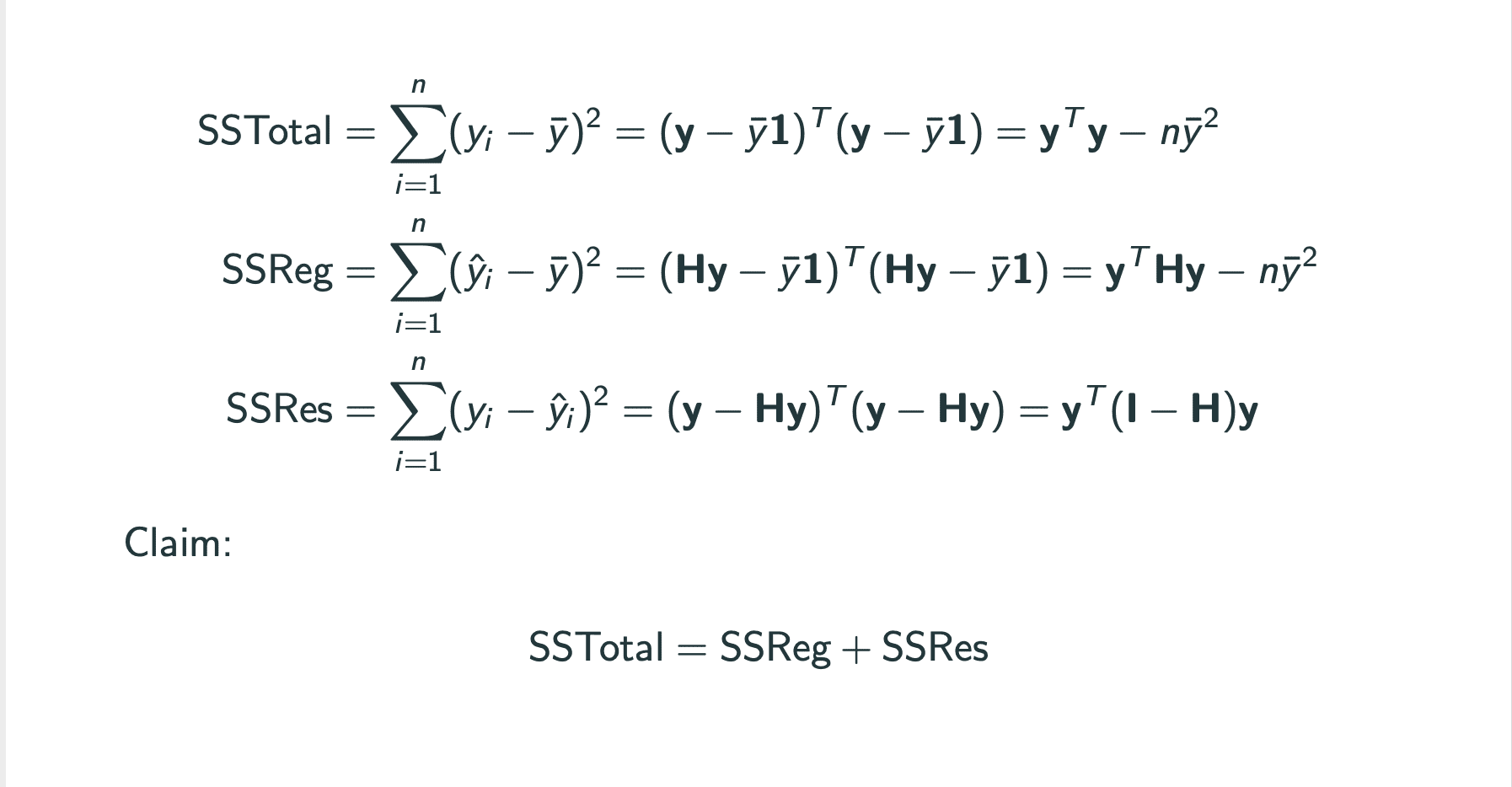
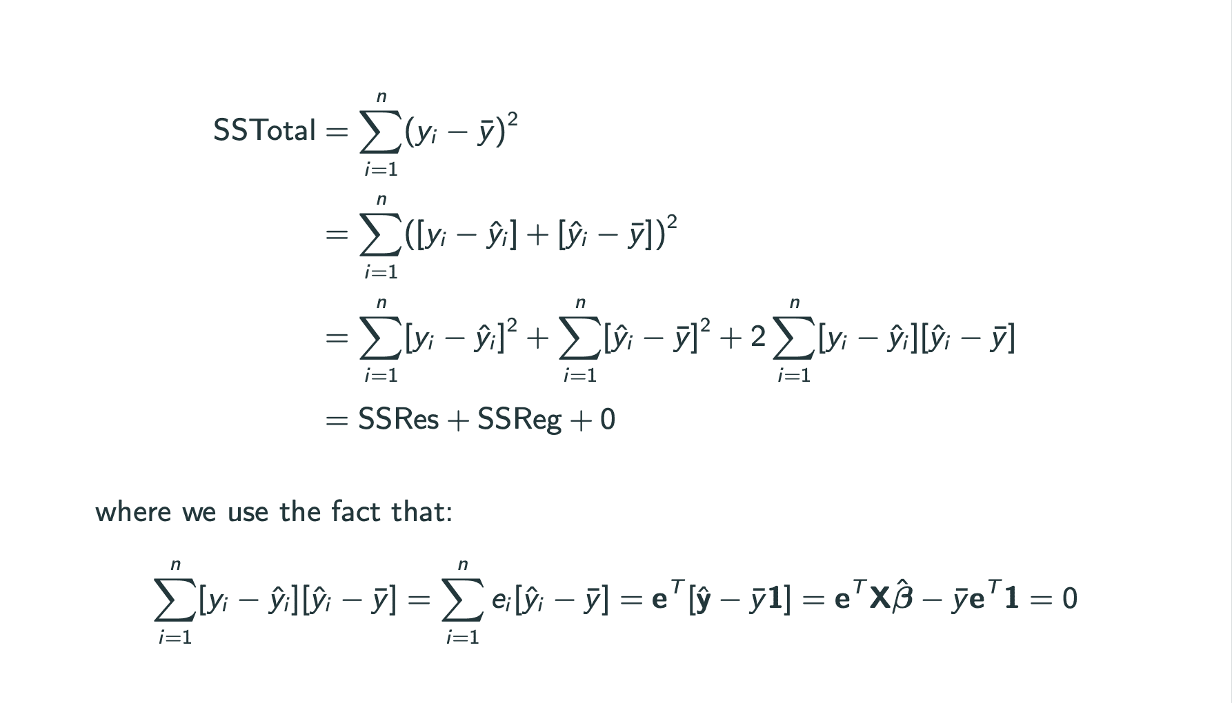
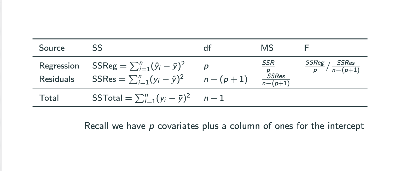
anova S S T O T = S S T R T + S S R E S SS_{TOT} = SS_{TRT} + SS_{RES} S S T O T = S S T R T + S S R E S
___
sampling
SRS
最大的区别是在公式中有finite population correction.
Example:model 1
confidence interval: μ : y ˉ ± c ∗ S n \mu: \bar{y} \pm \frac{c*S}{\sqrt{n}} μ : y ˉ ± n c ∗ S E = c ∗ σ 2 n E = \frac{c*\sigma^2}{\sqrt{n}} E = n c ∗ σ 2
Using SRS:μ : y ˉ ± 1 − n N c ∗ σ ^ n \mu: \bar{y} \pm \sqrt{1 - \frac{n}{N}} \frac{c*\hat{\sigma}}{\sqrt{n}} μ : y ˉ ± 1 − N n n c ∗ σ ^ E = 1 − n N c ∗ σ ^ n E = \sqrt{1 - \frac{n}{N}} \frac{c*\hat{\sigma}}{\sqrt{n}} E = 1 − N n n c ∗ σ ^
Example:model 4
with confidence interval: π : π ^ ± c ∗ π ^ ( 1 − π ^ ) n \pi: \hat{\pi} \pm c*\sqrt{\frac{\hat{\pi}(1-\hat{\pi})}{n}} π : π ^ ± c ∗ n π ^ ( 1 − π ^ )
Using SRS:π : π ^ ± c ∗ π ^ ( 1 − π ^ ) n 1 − n N \pi: \hat{\pi} \pm c*\sqrt{\frac{\hat{\pi}(1-\hat{\pi})}{n}}\sqrt{1 - \frac{n}{N}} π : π ^ ± c ∗ n π ^ ( 1 − π ^ ) 1 − N n
We have error 1 − n N c ∗ σ ^ n \sqrt{1 - \frac{n}{N}} \frac{c*\hat{\sigma}}{\sqrt{n}} 1 − N n n c ∗ σ ^ σ 2 ^ = π ^ ( 1 − π ^ ) \hat{\sigma^2} = \hat{\pi}(1-\hat{\pi}) σ 2 ^ = π ^ ( 1 − π ^ ) σ 2 ^ \hat{\sigma^2} σ 2 ^ π = 1 / 2 \pi = 1/2 π = 1 / 2
如何取sample size:
Take a small sample, estimate σ \sigma σ
Find n using formula.
Perform a large study with n units.
regression
regression sampling
Y i = α + β ( x i − ( ˉ x ) ) + R i Y_i = \alpha + \beta(x_i - \bar(x)) + R_i Y i = α + β ( x i − ( ˉ x ) ) + R i where R j ∼ N ( 0 , σ 2 ) R_{j} \sim N(0,\sigma^2) R j ∼ N ( 0 , σ 2 )
by least square:W = ∑ i r i 2 = ∑ i ( y i − α β ( x i − x ˉ ) ) 2 W = \sum_{i} r_{i}^2 = \sum_{i} (y_i - \alpha \beta(x_i - \bar{x}))^2 W = ∑ i r i 2 = ∑ i ( y i − α β ( x i − x ˉ ) ) 2 α ^ = y ˉ \hat{\alpha} = \bar{y} α ^ = y ˉ β ^ = S x y S x x = s x y s x x ^ \hat{\beta} = \frac{S_{xy}}{S_{xx}} = \frac{s_{xy}}{\hat{s_{xx}}} β ^ = S x x S x y = s x x ^ s x y σ r ^ 2 = W n − 1 \hat{\sigma_r}^2 = \frac{W}{n - 1} σ r ^ 2 = n − 1 W S x y = ∑ i ( y i − y ^ ) ( x i = x ˉ ) S_{xy} = \sum_i (y_i - \hat{y})(x_i = \bar{x}) S x y = ∑ i ( y i − y ^ ) ( x i = x ˉ ) s x y = S x y n − 1 s_{xy} = \frac{S_{xy}}{n - 1} s x y = n − 1 S x y S x x = ∑ i ( x i = x ˉ ) 2 S_{xx}= \sum_i (x_i = \bar{x})^2 S x x = ∑ i ( x i = x ˉ ) 2 s x x = S x x n − 1 s_{xx} = \frac{S_{xx}}{n - 1} s x x = n − 1 S x x
estimators: α , β , μ x , μ y \alpha, \beta, \mu_x, \mu_y α , β , μ x , μ y μ r e g ~ \tilde{\mu_{reg}} μ r e g ~ μ y \mu_y μ y
confidence interval: E S T ± c S E = μ r e g ^ ± c 1 − n / N σ r ^ n EST \pm c SE = \hat{\mu_{reg}} \pm c \sqrt{1 - n/N} \frac{\hat{\sigma_r}}{\sqrt{n}} E S T ± c S E = μ r e g ^ ± c 1 − n / N n σ r ^
1 2 3 4 5 6 7 8 9 10 11 12 13 attach( women) mean( height) mean( weight) set.seed( 1 ) sample_heights = sample( height, 5 ) mean( sample_heights) sd( sample_heights)
we can build SRS CI: μ h ^ ± c 1 − n N σ S R S ^ n \hat{\mu_{h}} \pm c \sqrt{1 - \frac{n}{N}} \frac{\hat{\sigma_{SRS}}}{\sqrt{n}} μ h ^ ± c 1 − N n n σ S R S ^
1
2
3
4
5
6
7
8
9
sample_weights = c ( 123 , 129 , 135 , 146 , 120 ) mean( sample_weights) plot( weight, height) sample_weights = sample_weights- mean( sample_weights) summary( lm( sample_heights~ sample_weights) )
The regression estimate is given by:
μ h e i g h t ^ = α ^ + β ( x i − x ^ ) = μ h e i g h t ( μ w e i g h t ) = 63.4 + 0.31 ( 136.7333 − 130.6 ) = 65.3 \hat{\mu_{height}} = \hat{\alpha} + \beta(x_i - \hat{x}) = \mu_{height}(\mu_{weight}) = 63.4 + 0.31(136.7333 - 130.6) = 65.3 μ h e i g h t ^ = α ^ + β ( x i − x ^ ) = μ h e i g h t ( μ w e i g h t ) = 6 3 . 4 + 0 . 3 1 ( 1 3 6 . 7 3 3 3 − 1 3 0 . 6 ) = 6 5 . 3 build regression CI: μ r e g ^ ± c 1 − n N σ r ^ n \hat{\mu_{reg}} \pm c\sqrt{1 - \frac{n}{N}}\frac{\hat{\sigma_{r}}}{\sqrt{n}} μ r e g ^ ± c 1 − N n n σ r ^
regression比SRS更接近.
___
ratio
ratio estimation
Y i = β x i + R i Y_i = \beta x_i + R_i Y i = β x i + R i where R i ∼ N ( 0 , x i σ 2 ) R_{i} \sim N(0,x_i \sigma^2) R i ∼ N ( 0 , x i σ 2 )
注,variance中乘了x_i,我们在计算的时候会计算x i x i 和 y i x i \frac{x_i}{\sqrt{x_i}}和\frac{y_i}{\sqrt{x_i}} x i x i 和 x i y i
by least square we have β ^ = y ˉ x ˉ \hat{\beta} = \frac{\bar{y}}{\bar{x}} β ^ = x ˉ y ˉ σ r a t i o ^ 2 = W n − 1 \hat{\sigma_{ratio}}^2 = \frac{W}{n - 1} σ r a t i o ^ 2 = n − 1 W μ r a t i o ^ = y ˉ x ˉ μ x \hat{\mu_{ratio}} = \frac{\bar{y}}{\bar{x}}\mu_x μ r a t i o ^ = x ˉ y ˉ μ x
with confidence interval: μ r a t i o ^ ± c 1 − n N σ r a t i o ^ n \hat{\mu_{ratio}} \pm c \sqrt{1 - \frac{n}{N}} \frac{\hat{\sigma_{ratio}}}{\sqrt{n}} μ r a t i o ^ ± c 1 − N n n σ r a t i o ^
1 2 3 4 5 6 7 8 9 10 11 12 13 14 15 16 17 18 19 20 attach( women) set.seed( 1 ) sample_heights = sample( height, 5 ) mean( sample_heights) sd( sample_heights) sample_weights = c ( 123 , 129 , 135 , 146 , 120 ) mean( sample_weights) plot( weight, height) Sqrt_weights = sqrt ( sample_weights) sample_weights = sample_weights/ Sqrt_weights sample_heights = sample_heights/ Sqrt_weights summary( lm( sample_heights~ sample_weights- 1 ) )
The ratio estimate is given by:μ h e i g h t ^ = β ^ ∗ x i = y ˉ x ˉ ∗ x i = 63.4 130.6 x i \hat{\mu_{height}} = \hat{\beta}*x_i = \frac{\bar{y}}{\bar{x}}*x_i = \frac{63.4}{130.6}x_i μ h e i g h t ^ = β ^ ∗ x i = x ˉ y ˉ ∗ x i = 1 3 0 . 6 6 3 . 4 x i
= 0.48545x_i.带入= 0.48545(136.7333) = 66.4
build regression CI: μ r a t i o ^ ± c 1 − n N σ r a t i o ^ n \hat{\mu_{ratio}} \pm c \sqrt{1 - \frac{n}{N}} \frac{\hat{\sigma_{ratio}}}{\sqrt{n}} μ r a t i o ^ ± c 1 − N n n σ r a t i o ^
ratio比SRS更接近.ratio是biased的.
proportion的情况下:
build regression CI:θ ^ ± 1 π ^ 1 − n N σ r a t i o ^ n \hat{\theta} \pm \frac{1}{\hat{\pi}}\sqrt{1 - \frac{n}{N}}\frac{\hat{\sigma_{ratio}}}{\sqrt{n}} θ ^ ± π ^ 1 1 − N n n σ r a t i o ^ σ r a t i o ^ = ∑ ( y i − θ z i ^ ) 2 n − 1 \hat{\sigma_{ratio}} = \sum\frac{(y_i - \hat{\theta_{zi}})^2}{n - 1} σ r a t i o ^ = ∑ n − 1 ( y i − θ z i ^ ) 2
θ ^ \hat{\theta} θ ^
___
stratified
计算subpopulation,每个subpopulation independent.
μ = N 1 μ 1 + N 2 μ 2 + . . . + N H μ H N = ∑ i = 1 H w i μ i \mu = \frac{N_1\mu_1+ N_2\mu_2 + ... + N_H\mu_H}{N} = \sum_{i = 1}^{H}w_i\mu_i μ = N N 1 μ 1 + N 2 μ 2 + . . . + N H μ H = ∑ i = 1 H w i μ i 这里的w是weight,也是占总人群的比例.
confidence interval: μ ^ ± c ∑ i = 1 H w i 2 σ i 2 n i ( 1 − n i N i ) \hat{\mu} \pm c \sqrt{ \sum_{i=1}^H w_i^2\frac{\sigma_i^2}{n_i}(1 - \frac{n_i}{N_i}) } μ ^ ± c ∑ i = 1 H w i 2 n i σ i 2 ( 1 − N i n i ) C ∼ N ( 0 , 1 ) C \sim N(0,1) C ∼ N ( 0 , 1 )
π = ∑ i = 1 H w i π i \pi = \sum_{i = 1}^{H}w_i\pi_i π = ∑ i = 1 H w i π i confidence interval: π ^ ± c ∑ i = 1 H w i 2 σ i 2 n i ( 1 − n i N i ) \hat{\pi} \pm c \sqrt{ \sum_{i=1}^H w_i^2\frac{\sigma_i^2}{n_i}(1 - \frac{n_i}{N_i}) } π ^ ± c ∑ i = 1 H w i 2 n i σ i 2 ( 1 − N i n i ) C ∼ N ( 0 , 1 ) C \sim N(0,1) C ∼ N ( 0 , 1 ) σ i 2 = π i ( 1 − π i ) \sigma_i^2 = \pi_i(1 - \pi_i) σ i 2 = π i ( 1 − π i )