为stat331附录的estimation相关代码.
Simple Linear Regression
我们通过Least Squares Estimation来estimate和.
(省略证明的步骤)
Maximum Likelihood Estimation和Least Squares Estimation估算的和是一样的.
当n大于50时,这两个没什么区别.
注:
同理
1 | #-------------------------------------------------------------------------- |
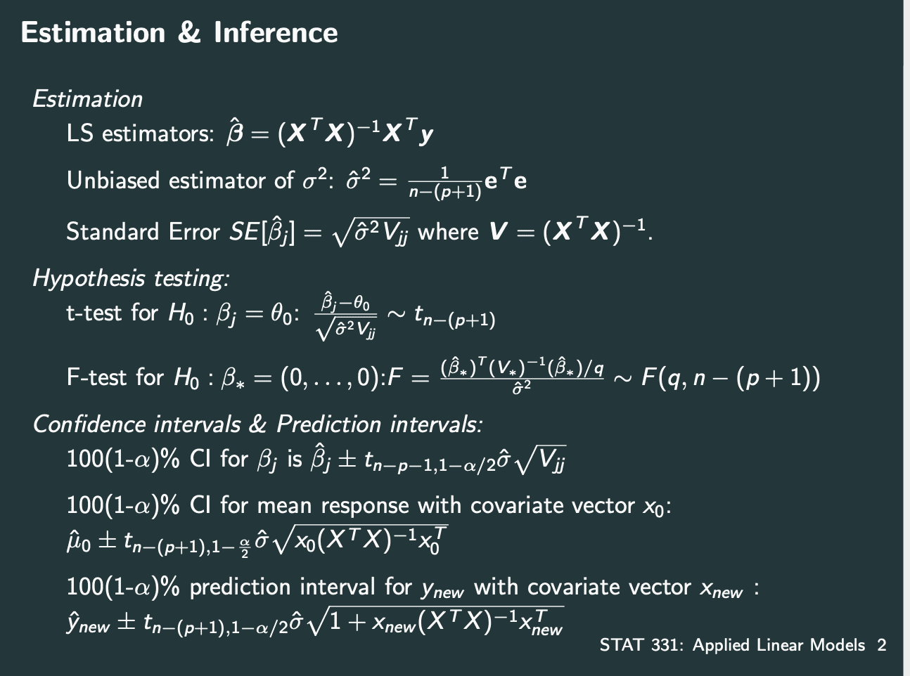
Confidence Intervals
注意confidence intervals分为知道sigma和不知道sigma.
知道sigma用normal distribution,不知道用t distribution.
通过MLE的distribution得知
在知道sigma的情况下,95%的
1.96是Z常数.
不知道sigma的情况下,我们使用,95%的
q由r计算.写作
1 | qt(p = 0.05/2, df = n-2, lower.tail = FALSE) |
虽然老师讲了很多的代码但不如直接用r自带的confint built-in function好了.
1 |
|
Hypothesis Testing
1 |
|
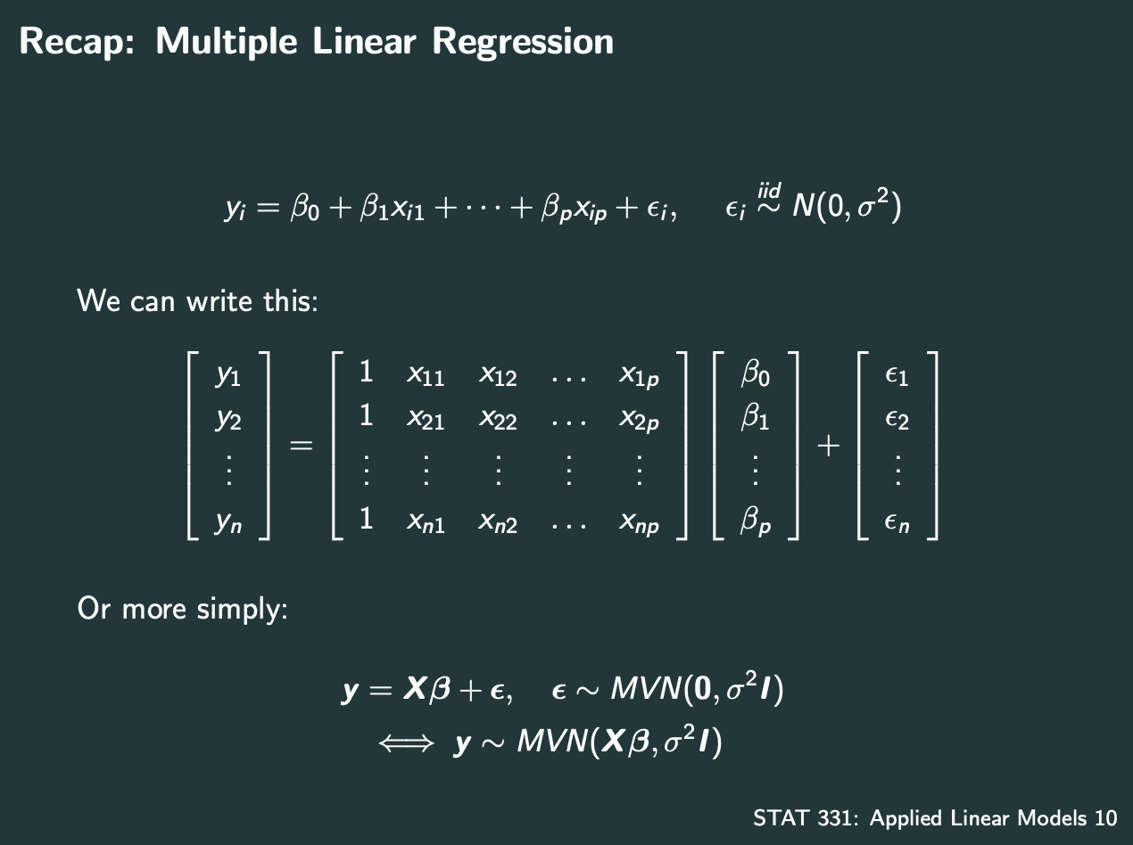
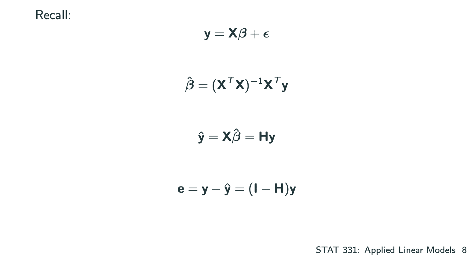
Multiple Linear Regression
也就是多个系数的model.
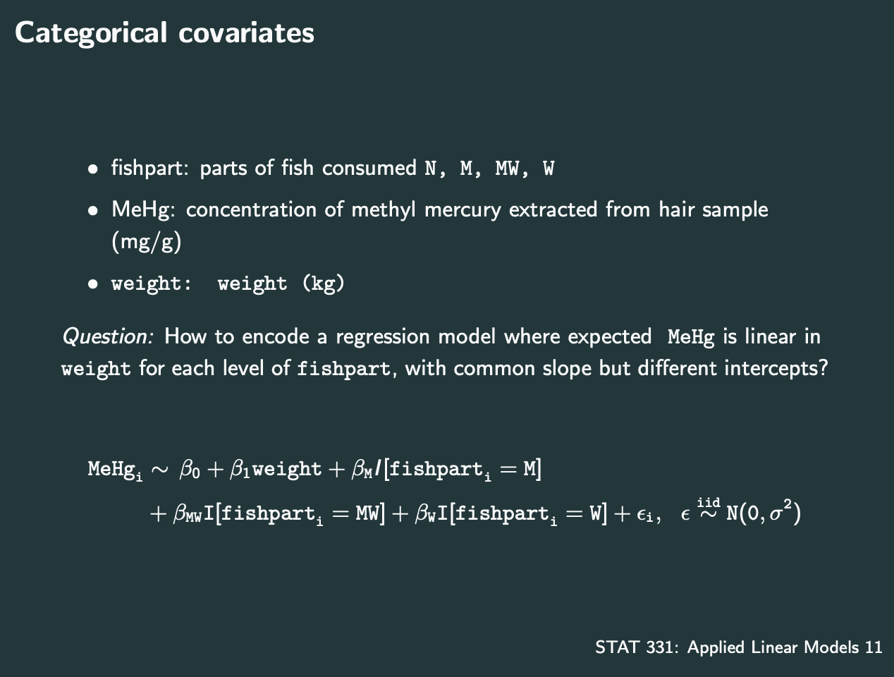
其中有系数是categorical的,需要特殊处理.
1 |
|
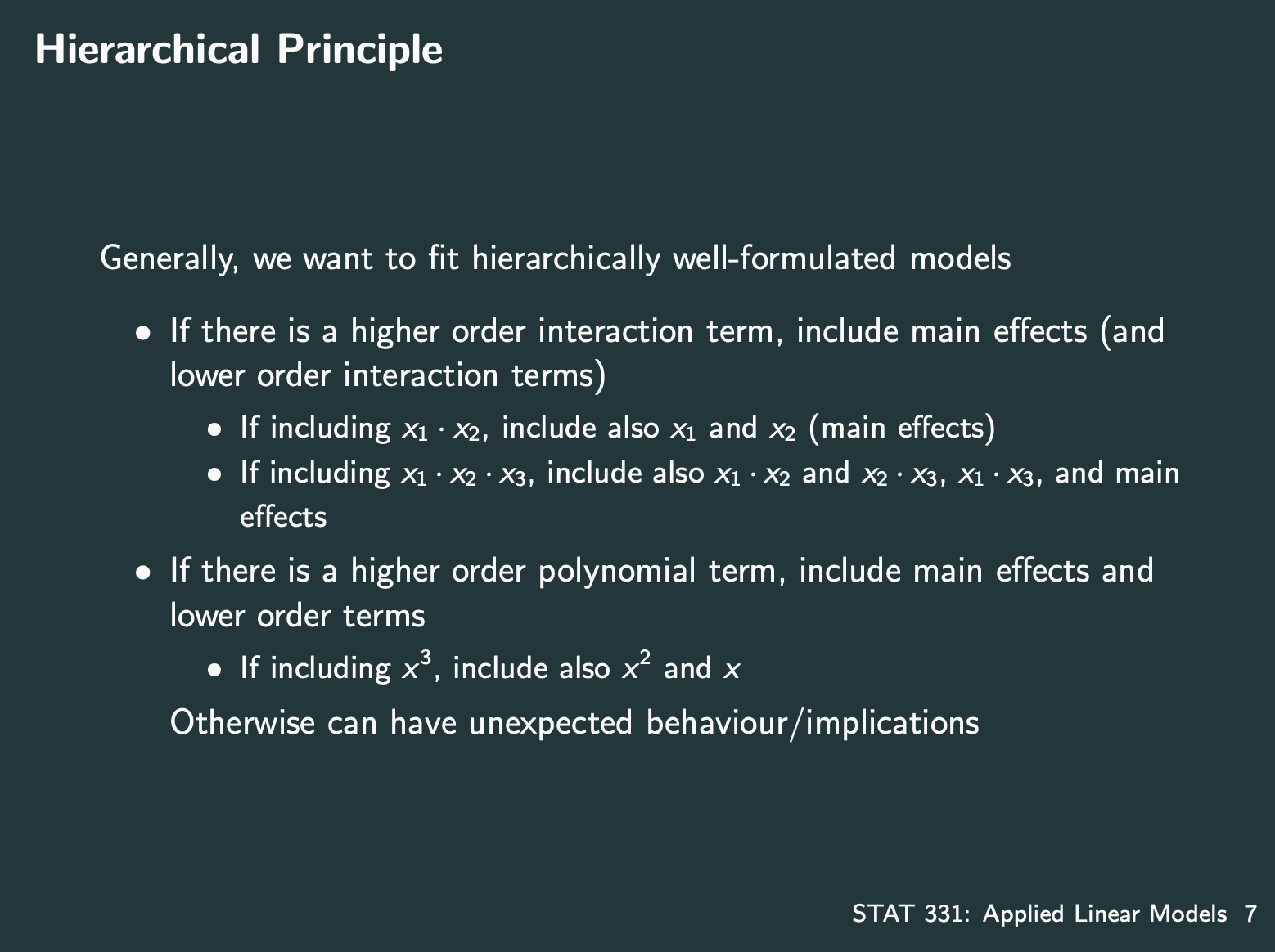
其中系数也可能有nolinear的情况.
插播stat444老师的名言:
all models are false but some are useful.
在Assignment1中的例子,按照scatter plot看出跟exponential像,所以plot exponential.
1 | log.sigma2.y = log(sigma2.y) |
1 | plot(Week.x, sigma2.y , pch=19, cex.axis = 1.5, cex.lab = 1.5, ylim=c(0,36000)) |
从R-squared中看出数据比较大(偏差比较大),model可以再优化.
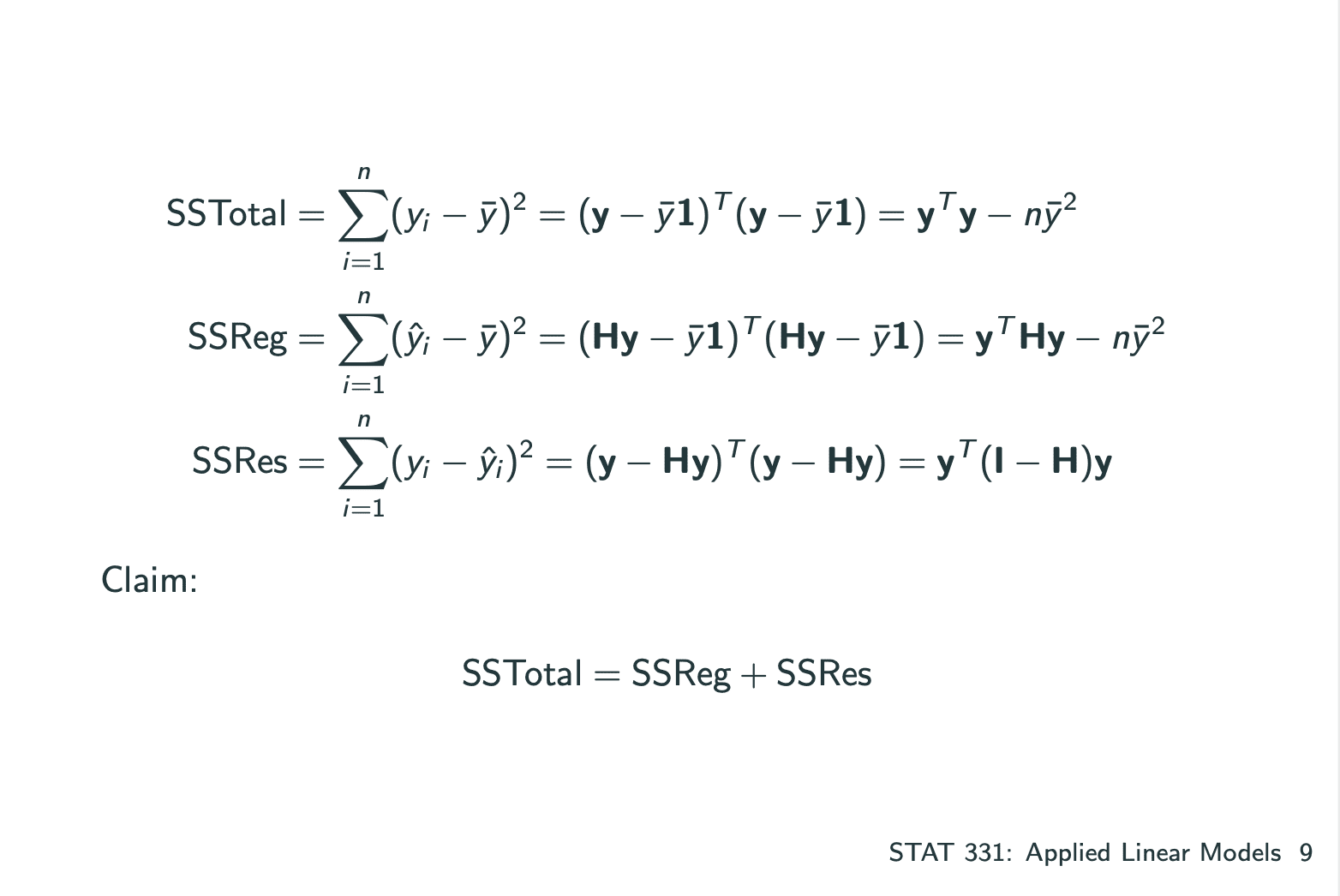
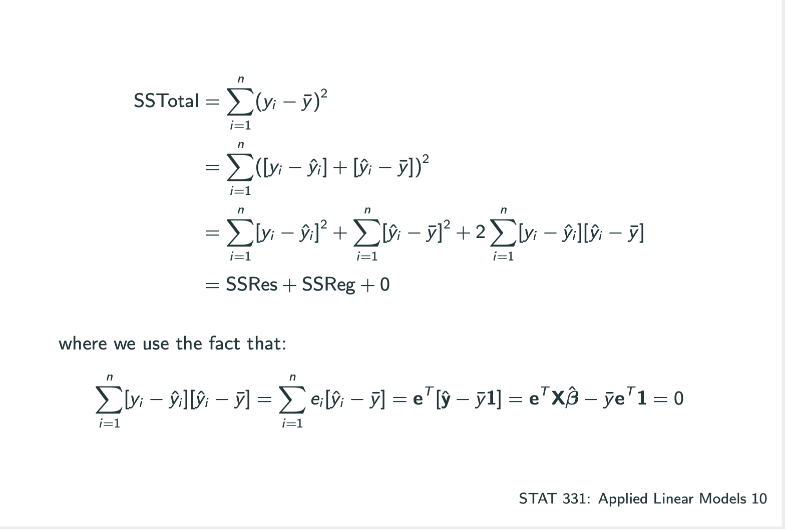
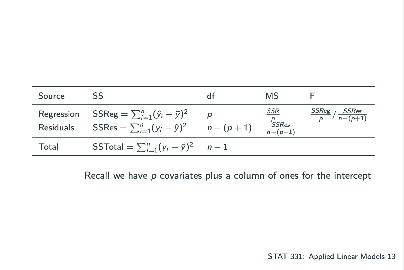
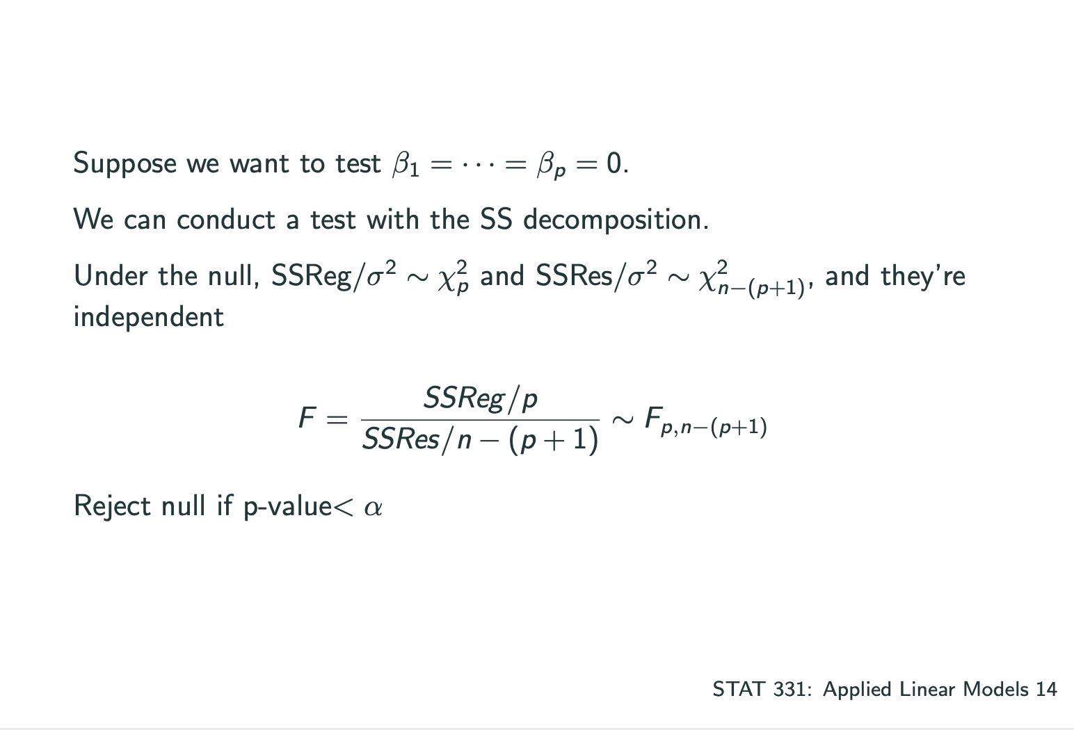
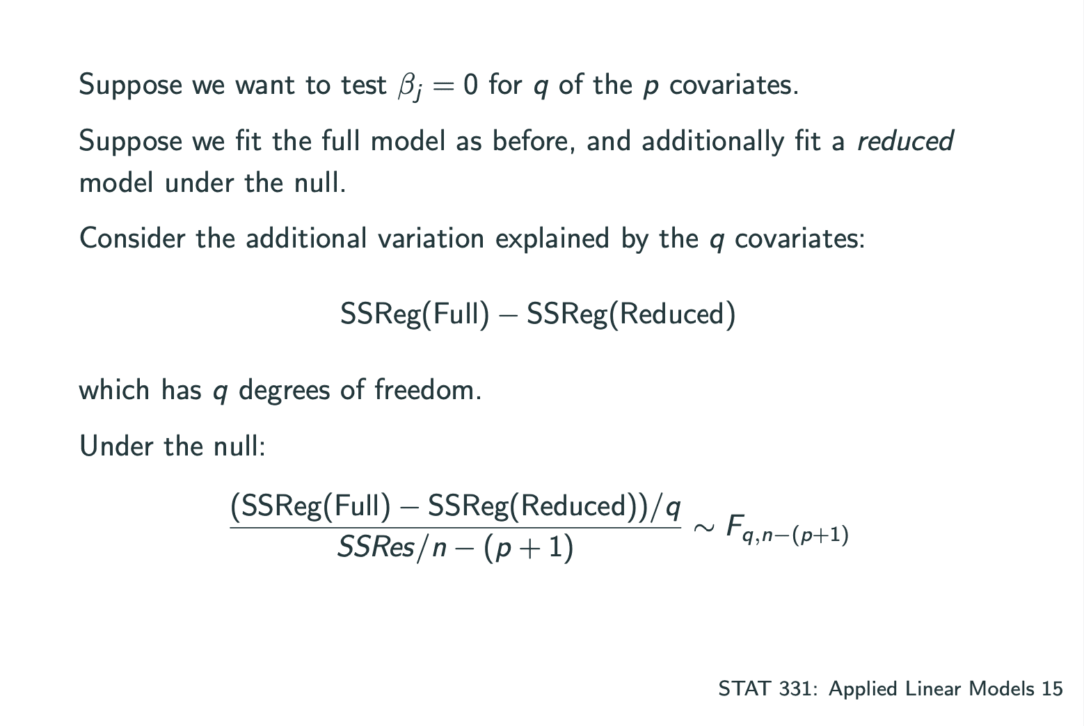
ANOVA
(这个在stat系列中有记载过,再次备份一下)
ANOVA: How much of the variability in Y is explained by our model?
1 | ### LECTURE 11 |
1 |
|
1 |
|
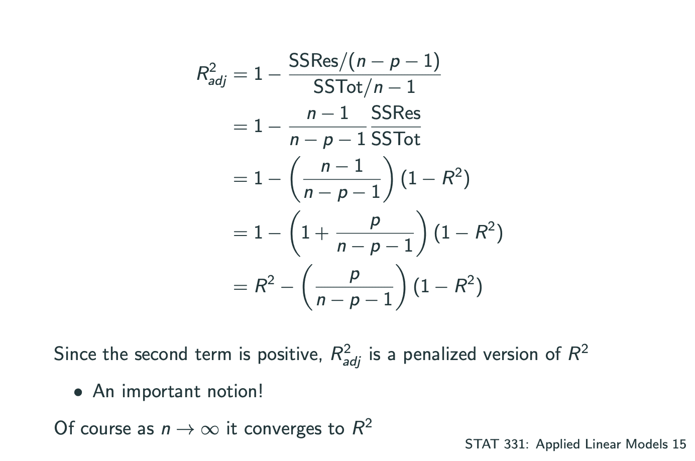
Goodness of Fit
测试一个model是否合适可以通过测试以下数据:
,where.Interpretation: proportion of variability explained by the model.
Problem: will never decrease when adding more variables.
因此可以测试Adjusted.
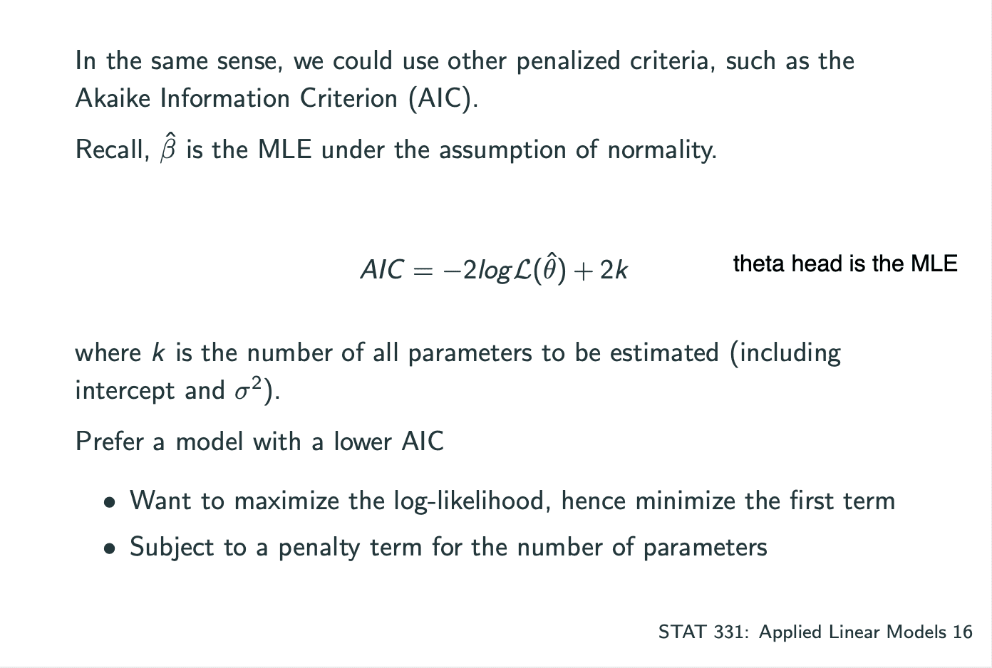
此外也可以测试AIC.
1 |
|
Automatic Selection
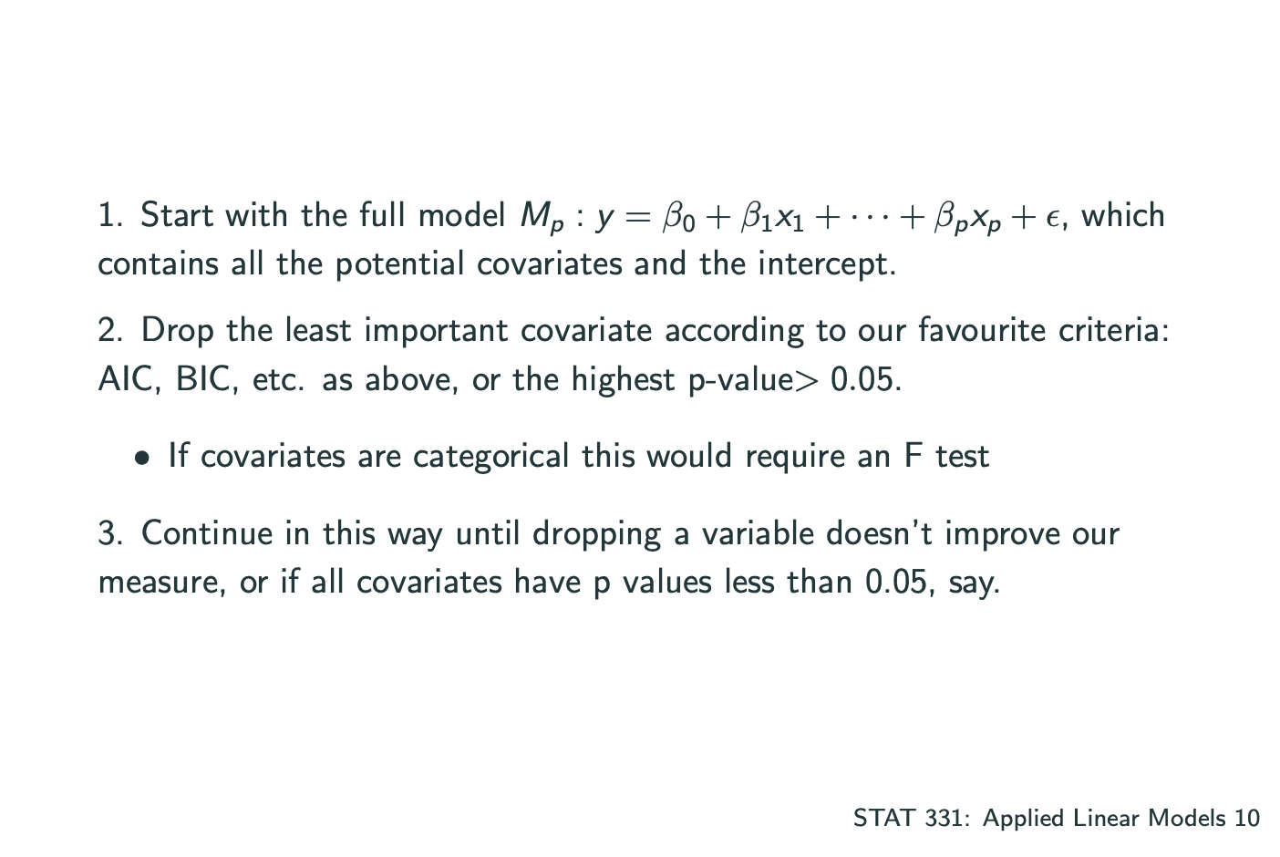
一个model中有多个系数,其中建立model的方式有 将所有的系数一个一个加入 和 一个一个减去 两种,分为Forward Selection和Backward Elimination.
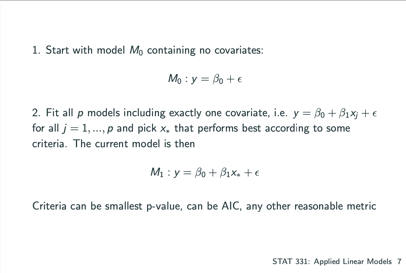
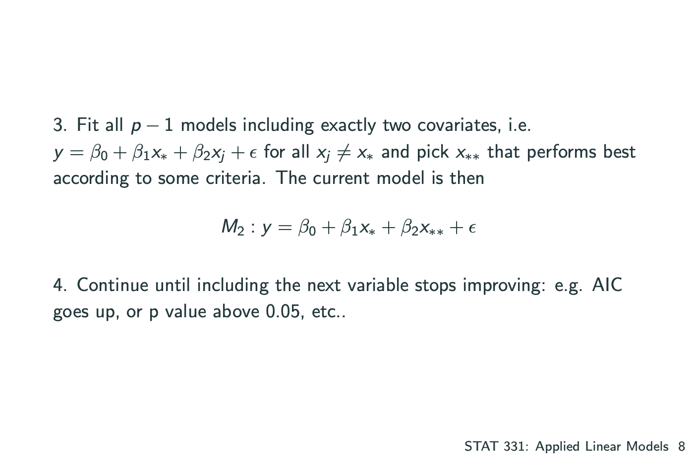
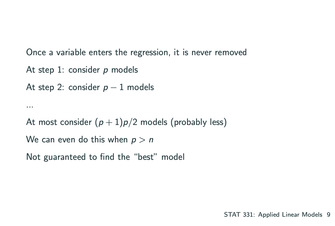
Forward Selection:
Backward Elimination:
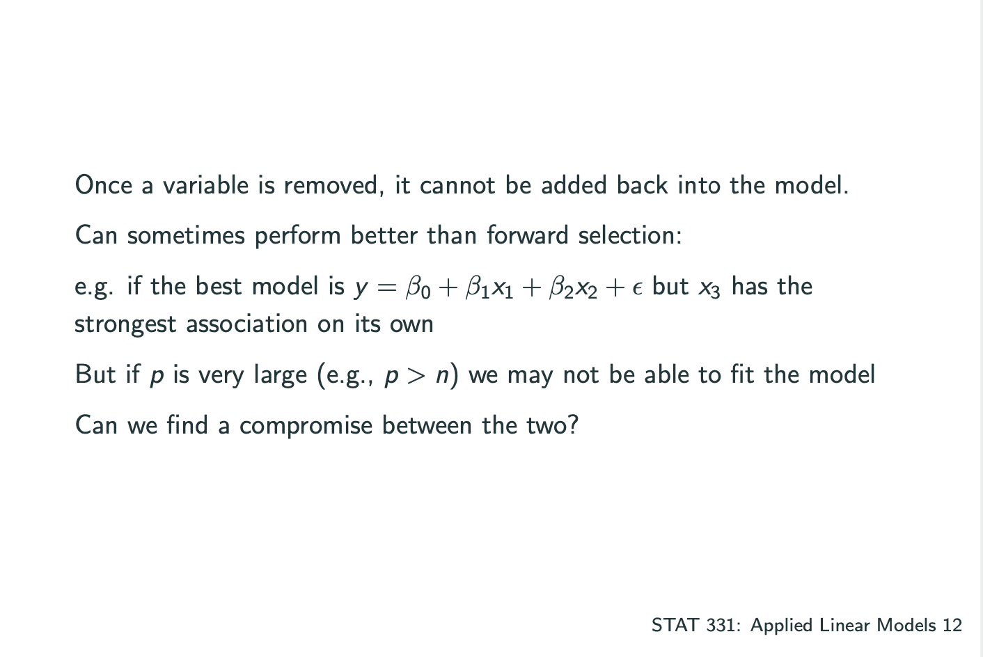
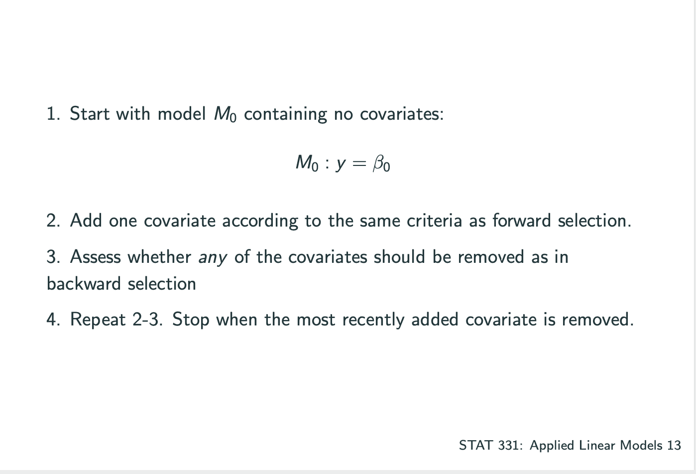
还有一种是combine了forward和backward,Stepwise Selection.
1 | # ------ automatic selection ------------------ |
Cross-validation
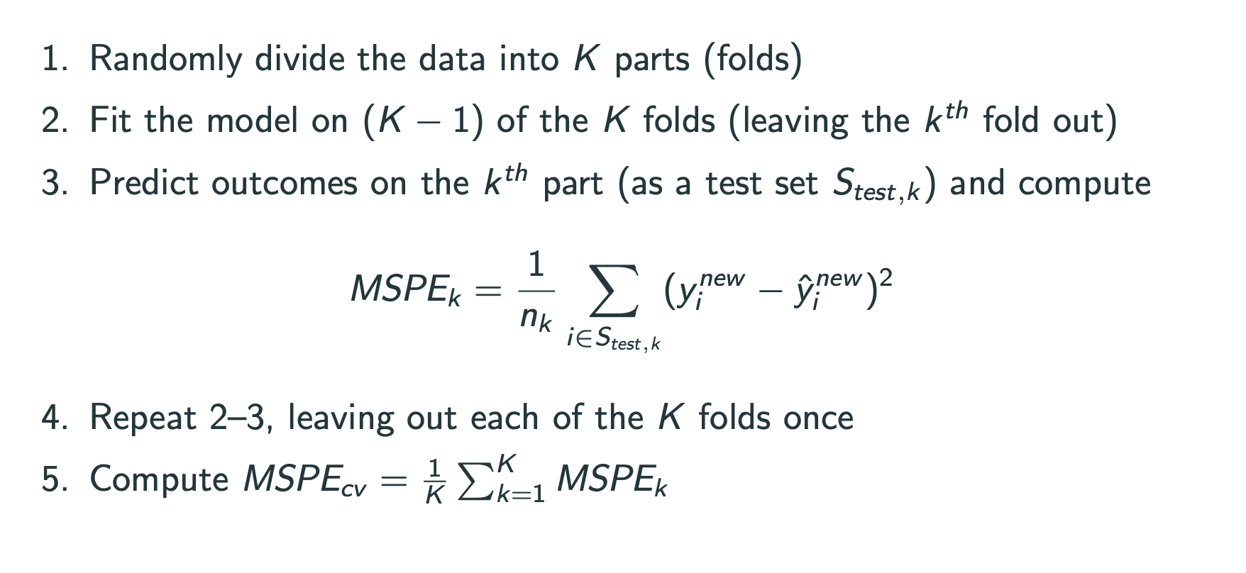
cross validation的思想是把数据分组,一部分作为training set,来fit model,一部分作为test set,用来测试fit的model的误差.
k-fold cross validation是其中的一种:将k-1组作为traning set.
leave-one-out cross validation则除了一个数据外将全部数据作为traning set,再计算其中的误差.
load data and fit models from lec 14:
1 |
|
1 |
|
1 |
|
k-fold cross validation stat444加强版:
这里也包括了LOOCV.
一般k-fold有更好的bais和variance trace off,但LOOCV会更快.
1 | # A function to generate the indices of the k-fold sets |
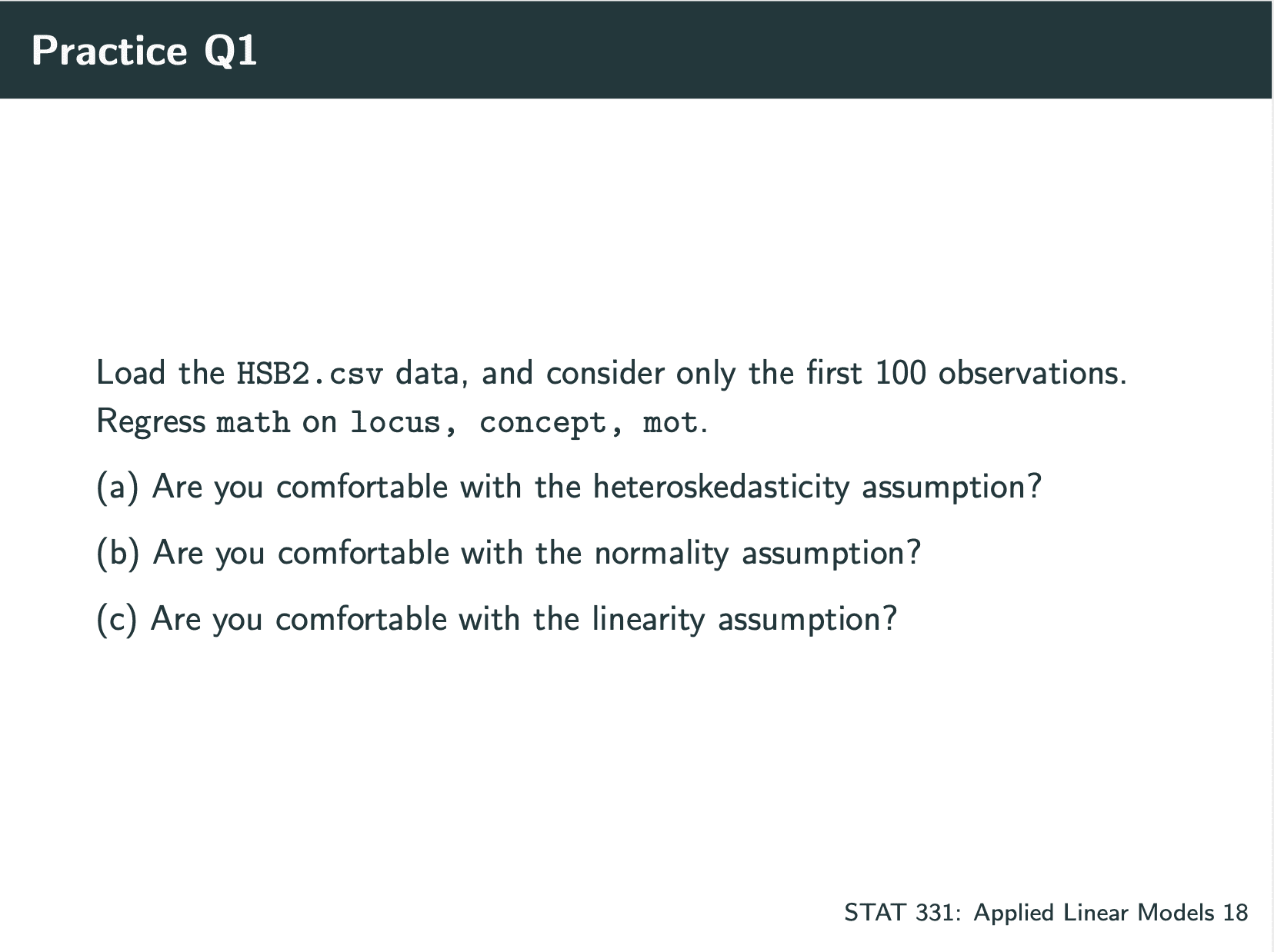
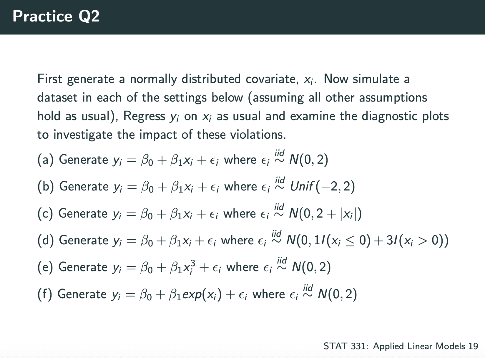
Linear Regression Assumptions:
- Linearity
- Independence
- Normality
- Equal variance (homoskedasticity)
code for checking them:
1 |
|
1 |
|
在不满足的情况下修改model:
- Linearity
- Instead include log(xj)
- Instead use a quadratic model (xj and xj2)
- Independence
- Estimates are still unbiased but standard errors are broken
=⇒ replace SEs with robust alternatives (sandwich form, GEE) - Explicitly model the dependence structure • Mixed effects models
- Normality
Violations of normality might not be a big deal
- E.g. if we have a large sample size
However, Normality is required for valid prediction intervals - Could consider transforming Y
E.g. model log(Y)
This again changes interpretations!
Might not be a problem if we’re interested in prediction - Could consider other regression approaches: GLMs, etc. (not covered in this course)
- Equal variance (homoskedasticity)
If our errors are heteroskedastic, we have a few options:
- Transform outcome (see above)
Variance stabilizing transform - Weighted Least Squares
- Bootstrap (time permitting…)
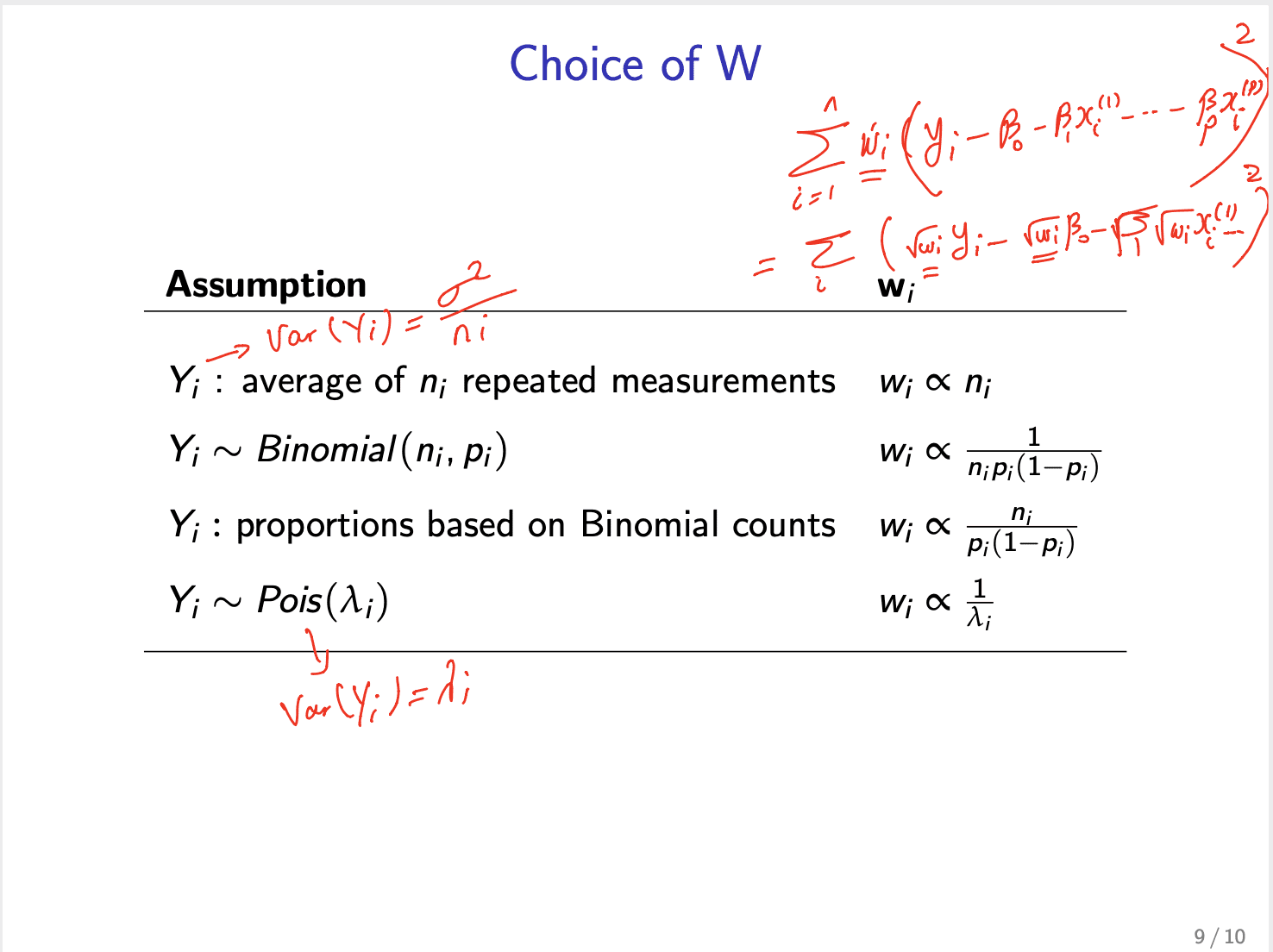
Weighted Least Squares:
1 | ## load packages |
1 |
|
stat444加强版选择weight: