
三次编辑版.以及添加VBA笔记.
Hotkey
Tips

常用功能可以右键放到quick access toolbar.
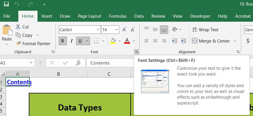 用dialogue box launcher to change text format.
execel自动format排版.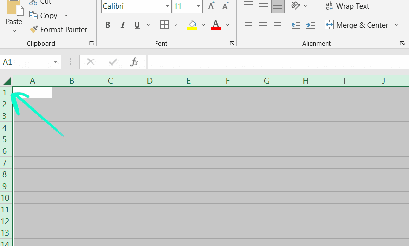
左上的小三角是全选,点击两个column/row之间的boundary可以自动排版.
我们可以hide the column.
顺便一提用自动排版会把hidden的column一键找出来.
小tip之group sheet.如果一个excel文件中有多个同排版的sheet,可以group后一起处理(比如字体格式变更).
整理数据时也可以用filter看表格中的数据一共有的类型.
Keys
ctrl+ home 可以快速回表格的A1.
快捷键F1 -> help
ctrl + Y -> redo
ctrl + drag -> make a copy
move -> just drag
move and insert a row -> shift + drag
我们可以set print area.在print前更改page layout.
ctrl + P -> print short key
(选中数据)alt + F1 -> create a column chart
alt + enter -> insert a new line within a cell
F11 key -> create chart in a separate sheet
alt + F11 -> a new chart embedded on the same sheet
ctrl + T -> inset a new table
sort in excel.
ctrl + A, 全选(会通过旁边是否有null的column来判断全表的内容)
ctrl + .(period) move the active cell around the corner of the range.
home tap有sort and filter, data tap里也有.
ctrl + shift + 8 -> 选择相近(包含)的active cell current region.
autofill,比较牛逼的一种自动检测sum.
short cut是 alt + =
Pivot table
关于pivot table.
可以快速计算table中的各个数据属性.
Row和Column是用来分析的数据属性,value是值.
比如我想知道countryside和city中的商品数据.
则按coutryside和city的location作为column,商品种类作为rows.
value可以选很多种,可以选任何一个column再选择count则是商品的贩卖数量,选总贩卖金额则是sum等.
最后加filters,用某个category的column来筛选数据.
注:可以在上方工具栏的design上选择subtotal选项.pivot table会默认给一个total,可以去掉.
ctrl + ⬆️ -> 最上的一行
ctrl + ⬇️ -> 最下的一行
要implement一整列的数据这样的快捷键很方便.
Rough notes
2022,Mar实习时的讲的function notes.
Function wizard
用来寻找function,by entering the functionality.
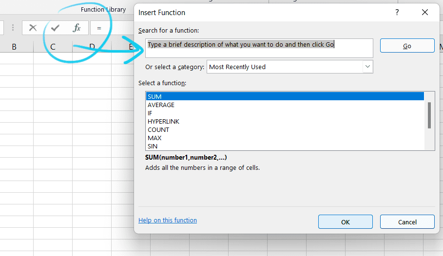
在function的icon里,可以用search使用function wizard.
然后直接用function arguments来使用function.
Networkdays
用来计算两个dates之间的非周末days,可以删掉hoilday.
例子:这个月有几个business day.
Networkdays(“01 Dec 2018”,”28 Dec 2018”)
Today()
reutrn today’s date.
PMT
Calcualte the payment.
Assumes a constant payment amount per payment period.
同类别的有FV, PV, RATE, NPV, IRR.因为自己跟financial一点都不沾边所以希望未来也不沾边…
Weekday
根据日期returns the day of the week. The day is given as an integer, ranging from 1 (Sunday) to 7 (Saturday), by default.
Replace
用来改string中的值,跟substitute不同的是需要从start_num和num_chars来锁定要替换的内容.
Name ranges
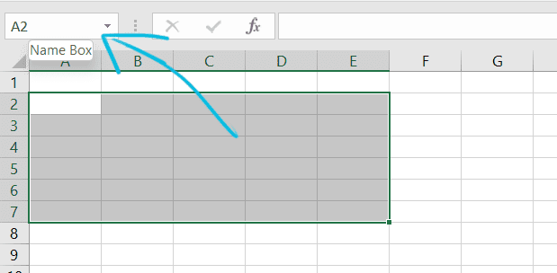
选中cell后可以直接edit此区域来给cell(可单数可复数)命名.注意命名不可以有空格.
命名后就可以用这块区域快速导向取过名的区域.
除此之外也可以在formulas > name manager里命名.
Table
我以为excel里面每个sheet上的内容就是table了而并不是,table在excel里是种的data type.
Convert data to table:选中你的数据, insert > table.
当数据的格式/颜色变了,就变成了table.
Table还智能,在旁边加数据,自动会变为table的一部分.
当数据成table后,选中就会多处一个table design的tab.

Data validation
一个很牛逼的,提前编辑cell内值的功能.
Any number between 501 and 1000:
Data > data validation > data validation > setting > allow whole number > between
这样就只能输入501到1000的数字,如果输入其他的会报错并阻止.
也可以只跳出warning instead of error.
Any number greater than 300 + user can over-ride with other entries:
Data > data validation > data validation > setting > allow whole number > greater than
Select input message to enter your message
Select Error Alert > style > warning or information > enter an error message
如果要用categorical data的情况:
首先每种选择都得在不同的cell中.还可以增加一个input message.
然后Data > data validation > data validation > setting > list > source选中刚刚准备好的cell.
Text to column
如果遇上一个cell里有”A,B,C”可以用此功能变成三个cell分别放A,B和C.
Press ctrl + A 全选,再Data > Text to column.
Sort
虽然data > filter功能也有自带sort.
Filter里的sort是默认AtoZ或者ZtoA,用data > sort里可以加不同的level,先用index sort(一个level),再用industry sort(又一个level).
也使用Home tab sort and filter.
Proper
原来还有这么一个check capitialize的function
taXI -> Proper(taXI) -> Taxi
其他常见的all in lower case: lower, all in upper case: upper, trim unnecessary spaces: trim.
Ref
传说中$,用来酌情锁定数据.
B5:Column not fixed, row not fixed
$B5:Column fixed, row not fixed
B$5:Column not fixed, row fixed
$B$5:Column fixed, row fixed
不过在table中就不使用$而使用@了.
linking to a cell in the same table: [@[ColumnName]]
Linking to a cell in a different table : TableName[@ColumnName]
fix column: TableName[[ColumnName]:[ColumnName]]
fix cell: TableName[@[ColumnName]:[ColumnName]]
F4快捷键:
Clicking on one part of the formula and then pressing F4 changes just that part of the formula. The select the next part of the formula to change and start pressing F4 again.
F2 + ctrl + enter: fill a range easily.
用Ref的时候可以把一些储存constant的cell先取名,然后用named range指定cell,可读性更高.
Count
Count和counta的区别:
Count只能读numerical的数据,counta可以mix numerical和text.
Countif可以用输入string来计算categorical的数据,没想到比较数字大小也是用string扩起来的().
(这算是比较string的大小,还是比较numerical的大小啊)
=Countif(range,”>5”)
就是数字比5大的个数.
当然这里的“>5”也可以写在某个cell里做cell reference.
顺便一提averageif跟countif不同.
Countif“选取比较范围”和“计算数据”是一样的.
Averageif就得”选取比较用范围”,“比较用condition”,再加上计算的数据.
类似的function有:
Countif / Countifs
Averageif / Averageifs
Minifs
Maxifs
sumif(range,criteria,sum_range)
第一组是matching用的key value们,criteria是matching condition(return bool),最后的sum_range才是要sum的计算用数据.
又其中普通数据和table数据的比较时输入格式有不同,不过excel会自动handle,谢谢你excel.
Sumproduct
如字面所说.结合sum和product.
If
是我们的老朋友if else condition.
不过excel是以if()为function来运作的.
如果要if套if,就得function套function,看着有点胃疼…
If同系列有,
- 作为辅助的And和Or
- Iferror
If的function为:
=If(cell<condition,”true”,”false”)
如果要在三个condition中选择,得用两个if.
其中小于的(<)可以替换成不同,<>为不等于.
And和Or return boolean.
=If(And(cell<condition,cell>condition),”true”,”false”)
一个trick.
在if想要输出的,”true”和”false”情况的string,可以做加法.
比如:”there is a risk of “&cell.那橘子就会变成“there is a risk of” + cell value.
Iferror的用法是在if function外套一层,如果报错则显示error message.
iferror(averageif(range,condition,value),”error message”)
Lookup
除了学习过的vlookup外,还有hlookup,index,match.
=vlookup(lookup_value,table_array,col_index_num,[range_lookup])
Range_lookup: exact match = false; approximate match = true
True时, each boundary must be in sequential order, the data must be sorted in ascending order.
Col_index_num:想要的value的index.
Restriction: Order is look to the right, first come first serve.
=index(array,row_num,[column_num])
look inside a table in any direction to pull off a value.
很直爽的,从array(表格数据)中按row&column number来找值的function.
=match(lookup_value,lookup_array,[match_type])
calculates the position number of a value,经常跟lookup混合使用.
用于lookup/match中的index num一项.
Match_type: 0, exact match; 1, less than; -1, greater than.
Cell formatting
可以自定义formatting,比如Negative as red.
Round up and round down
Concatenate
Combine string.
顺便一提遇到了用concatenate,combine一个0.50%的cell,但combine时读取成了0.5023421这样的格式.
于是增加了text function来帮忙先convert.
Btw replacing items we can do substitute.
Chart
三种create chart:
- auto-detect(insert > chart)
- tweak
- build from scratch

当有chart后,就可以在chart design中更改格式等等.
在图片想要更改的区域右键或双击也能更改design.
(比如双击y轴就可以输入bound中的min和max,更改unit)

能调的东西很多,比如scattor plot想用圆圈和方块,在series option中找到数据组,再用marker调.
手动创建chart,可以先选中空白的地方造一张空白的图.
再右键空白表格,select data添加数据.
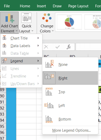
手动更改chart,举例Legend Entries.
Conditional formatting

在多个规则时可以调整priority.
Sparklines
A mini-chart in one cell that relates to a row of data.
Pivot table
是我们的老朋友pivot table.
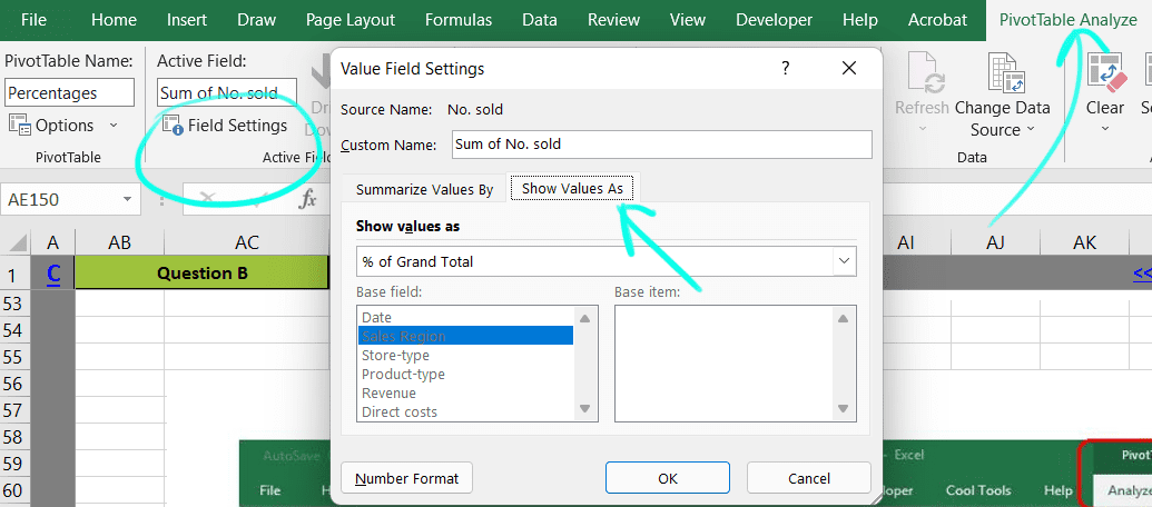
有的时候自动的field setting叫不出来,原来可以在ribbon手动设置.
包括show value as.
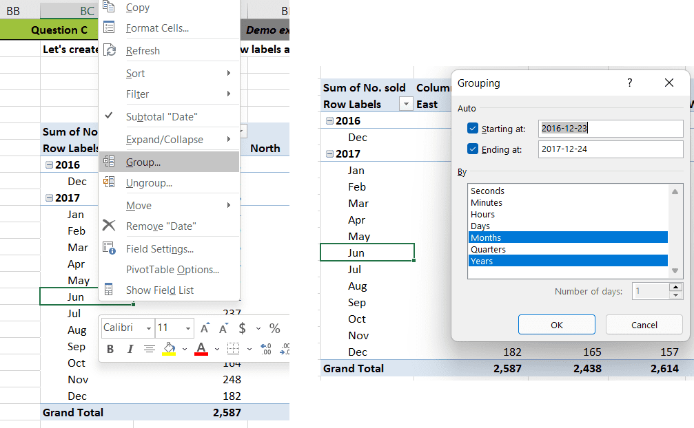
正确的grouping方式.
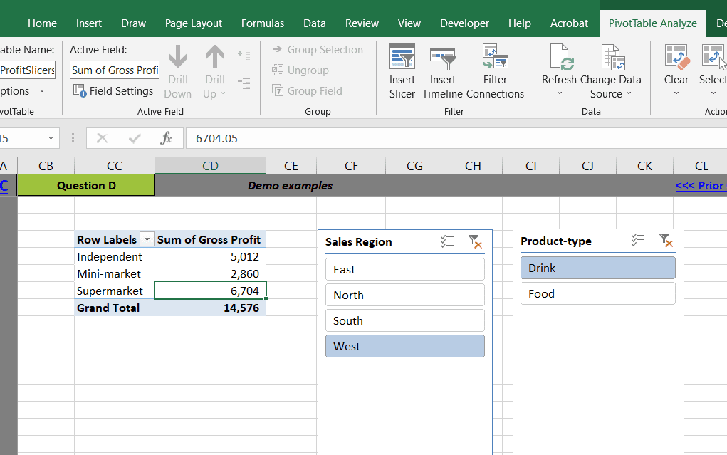
跟filter类似的silcer功能. Analyze -> insert slicer.
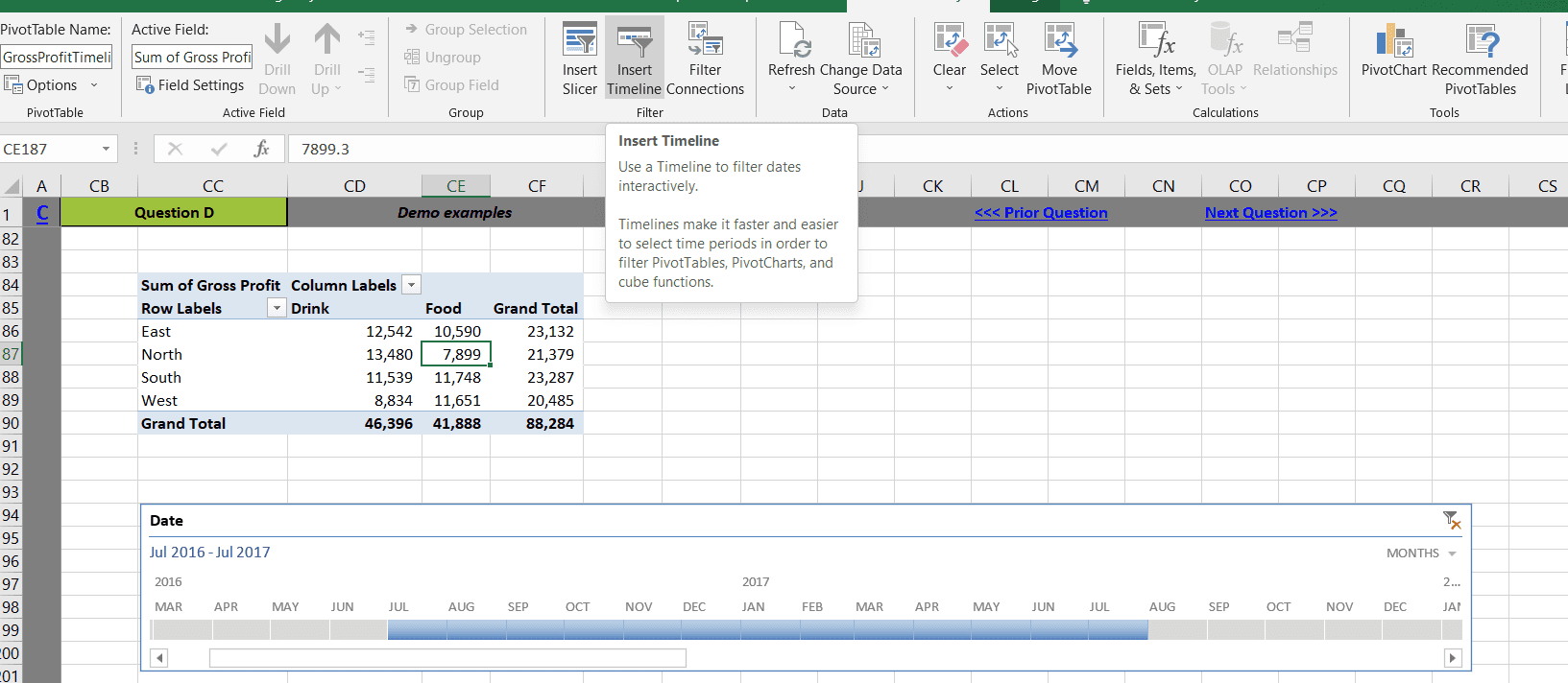
还有一看就很牛逼的timeline功能.
还可以手动添加一个column value,不需要在原表格上动手脚了!
Pivot chart跟普通的chart区别:因为跟pivot table链接,所以在table中filter数据,pivot chart也会变化,会方便.
What-If analysis
Data -> What-if analysis -> Goal seek/Solver
Goal Seek
Seeking a certain end result and require excel to change one of the input variables.
Can have many input variables but model one variable at a time.
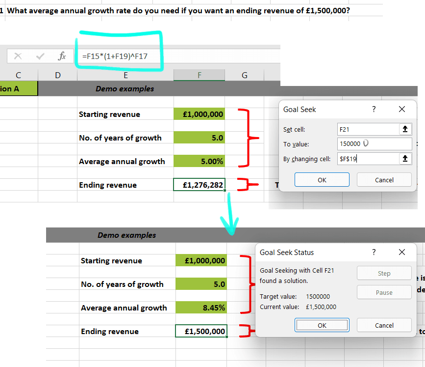
某种意义的一元方程式求解用功能.选中某个已经有formula的cell中,输入想要的结果和可以变的variable,goal seek来求出variable的值.
Solver
Modelling more than one input variable, solver will optimize the solution by finding the best combination of input variable.
Solver需要手动添加.
File -> options -> add-ins -> solver add-in -> click go -> check solver add-in
Then in data tab the most right, you have solver.
Solver可以做LP啊牛逼.
LP有机会也整理个笔记吧,那可是我滑铁卢黑暗回忆的经典篇章.
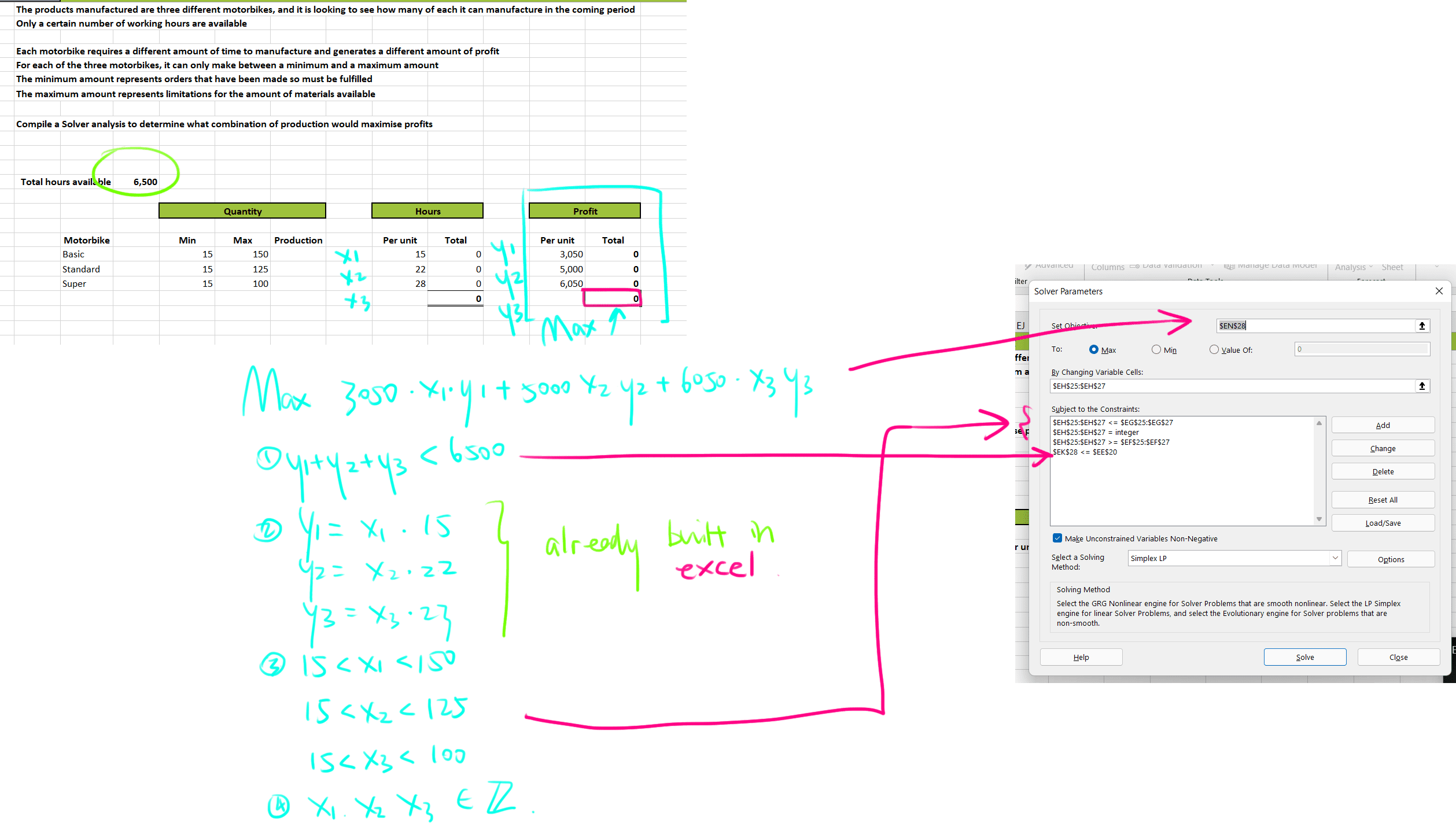
虽然我自己写的时候设了x1和y1组.但y1是依赖于x1的假variable,是LP没错.
solver的使用不单单要built-in,像这个例子中,excel里已经设置好了y1的计算,y1+y2+y3的和,profit sum,这样才能在有限的contraints function里表达出所有的式子.
Quiz
来自于2021,Nov18收到的测试题.考的是基本操作,搜到的方法收集如下.
- Highlight all Numbers greater than 80. 使用Conditional formatting.
同理的题目:
我有“FirstName LastName”格式的string,例如“Donna West”,我要cut出First name和Last name.
LEFT(B5,FIND(“ “, B5) - 1)
假如value在B5.用Find找出空格的位置,用LEFT可以得到从左到右的部分.同理用RIGHT就能得到Last Name.
Substring between parentheses
To extract a substring between parentheses (or braces, brackets, slashes, etc.), use MID and FIND in Excel.
- The formula below is almost perfect.
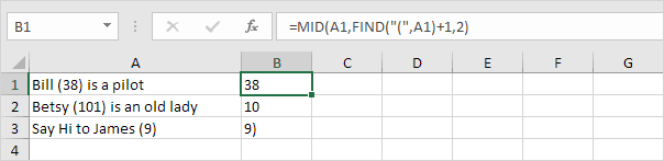
Explanation: the FIND function finds the position of the opening parenthesis. Add 1 to find the start position of the substring. The formula shown above reduces to MID(A1,6+1,2). This MID function always extracts 2 characters.
- Replace the 2 (third argument) with a formula that returns the length of the substring.
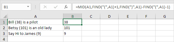
Explanation: subtract the position of the opening parenthesis and the value 1 from the position of the closing parenthesis to find the correct length of the substring.
Combine data using the CONCAT function
Select the cell where you want to put the combined data.
Type =CONCAT(.
Select the cell you want to combine first.
Use commas to separate the cells you are combining and use quotation marks to add spaces, commas, or other text.
Close the formula with a parenthesis and press Enter. An example formula might be =CONCAT(A2, “ Family”).
How to Use Excel to Match Up Two Different Columns
Use conditional formatting: new rule -> Use a formula to determine which cells to format.
= countif($C:$C, $A2)Date
- Sumifs + rolling time sum
Sumif和Sumifs是两个function,parameter有少许不同!
我所写的,check通patient ID + rolling time period计算方式.
=SUMIFS(K:K, C:C, “>=” & DATE(YEAR(C2),MONTH(C2),DAY(C2)-180), C:C, “<” & DATE(YEAR(C2),MONTH(C2),DAY(C2)),A:A,”=”&A2) + SUMIFS(K:K, C:C, “=” & C2,A:A,”=”&A2)
*疑惑之,在sql写self-join的时候,会有两个条件.“比自己大”+“比预计时间小”,翻找的例子却没有.
可能是例子默认“日期顺序已经被排列好了”.我的数据并没有,所以查询的row范围也是“那一column的全部”.