
两周的笔记一起摸,不愧是我.
DA的过程
question -> wrangle -> explore -> draw conclusion -> communicate
wrangle:
- gather data
- assess data to identify problems
- clean data(modify, replace, move to ensure data is high quality and well-structured)
explore:
- finding patterns
- visualizing relationship
- building intuition
- remove outliers
- create new and more descriptive features
draw conclusion:
- and make prediction
communicate:
- 也是最重要的(…)
- data visualization is very valuable
more CSV with Jupyter Notebooks
matplotlib
关于用matplotlib画图.
example
1 | import matplotlib.pyplot as plt |
another example
1 | # Use query to select each group and get its mean quality |
seaborn
用seabron画图.
example
1 | import seaborn as sns |
examples
1 | import numpy as np |
sciPy
用sciPy算数学相关_.
random
1 | import numpy as np |
如果我们要一次进行多组数据,使用array,比如说一次扔三次硬币,重复多次.
1 | # simulate 1 million tests of three fair coin flips |
binomial
1 | import numpy as np |
注:如果我们的数据在一个array里,我们可以用arr.mean()来计算mean.同理也有arr.std()和arr.var()可以计算standard deviation和variance.
练习notes
Pandas
A column in a df has boolean True/False values, but for further calculations, we need 1/0 representation. How would you transform it?
用astype(int)来转换.
1 | df["somecolumn"] = df["somecolumn"].astype(int) |
Describe how you will get the names of columns of a DataFrame in Pandas?
1 | list(data.columns) |
How are iloc() and loc() different?
这个我会!loc需要的key的值,而iloc是index number.
How can you sort the DataFrame?
用DataFrame.sort_values().
1 | #Sort by col1 |
How can you find the row for which the value of a specific column is max or min?
1 | df['A'].idxmax() |
This return column index.
How to split a string column in a DataFrame into two columns?
Use str.split.
1 | df[['code','location']] = df['row'].str.split(n=1, expand=True) |
How to check whether a Pandas DataFrame is empty?
1 | if df.empty: |
How would you iterate over rows in a DataFrame in Pandas?
1 | import pandas as pd |
Compare the Pandas methods: map(), applymap(), apply()
The map() method is an elementwise method for only Pandas Series, it maps values of Series according to input correspondence.
It accepts dicts, Series, or callable. Values that are not found in the dict are converted to NaN,
1 | # Example: |
The applymap() method is an elementwise function for only DataFrames, it applies a function that accepts and returns a scalar to every element of a DataFrame.
It accepts callables only i.e a Python function.
1 | # Example: |
The apply() method also works elementwise, as it applies a function along input axis of DataFrame. It is suited to more complex operations and aggregation.
It accepts the callables parameter as well.
The applymap() method is an elementwise function for only DataFrames, it applies a function that accepts and returns a scalar to every element of a DataFrame.
It accepts callables only i.e a Python function.
1 | df = pd.DataFrame([[4, 9]] * 3, columns=['A', 'B']) |
Describe how you can combine (merge) data on Common Columns or Indices?
Using .merge() method which merges DataFrame or named Series objects with a database-style join. You have inner, left, right and outer merge operation.
By default, the Pandas merge operation acts with an “inner” merge. An inner merge, keeps only the common values in both the left and right dataframes for the result.
Left merge, keeps every row in the left dataframe. Where there are missing values of the “on” variable in the right dataframe, it adds empty / NaN values in the result.
Right merge, keeps every row in the right dataframe. Where there are missing values of the “on” variable in the left column, it adds empty / NaN values in the result.
A full outer join returns all the rows from the left dataframe, all the rows from the right dataframe, and matches up rows where possible, with NaNs elsewhere
How can I achieve the equivalents of SQL’s IN and NOT IN in Pandas?
Use pd.Series.isin.
For IN use: something.isin(somewhere)
1 | df[df['A'].isin([3, 6])] |
For NOT IN: ~something.isin(somewhere)
1 | df[-df["A"].isin([3, 6])] |
How do you split a DataFrame according to a boolean criterion?
We can create a mask to separate the dataframe and then use the inverse operator (~) to take the complement of the mask.
1 | import pandas as pd |
How would you convert continuous values into discrete values in Pandas?
Depending on the problem, continuous values can be discretized using the cut() or qcut() function:
cut() bins the data based on values. We use it when we need to segment and sort data values into bins evenly spaced. cut will choose the bins to be evenly spaced according to the values themselves and not the frequency of those values. For example, cut could convert ages to groups of age ranges.
qcut() bins the data based on sample quantiles. We use it when we want to have the same number of records in each bin or simply study the data by quantiles. For example, if in a data we have 30 records, and we want to compute the quintiles, qcut() will divide the data such that we have 6 records in each bin.
How would you create Test (20%) and Train (80%) Datasets with Pandas?
scikit learn’s train_test_split is a good one - it will split both numpy arrays as dataframes.
1 | from sklearn.model_selection import train_test_split |
Name some type conversion methods in Pandas:
- to_numeric()
provides functionality to safely convert non-numeric types (e.g. strings) to a suitable numeric type. - astype()
convert (almost) any type to (almost) any other type. Also allows you to convert to categorial types (very useful). - infer_objects()
a utility method to convert object columns holding Python objects to a pandas type if possible. It does this by inferring better dtypes for object columns. - convert_dtypes()
convert DataFrame columns to the “best possible” dtype that supports pd.NA (pandas’ object to indicate a missing value).
Pivot Table Challenge
To provide the required df we use the function pivot_table with the parameters index=’Col X’, columns=’Col Y’ and as aggfunc, len:
1 | pd.pivot_table(df, index=['Col X'], columns=['Col Y'], aggfunc=len, fill_value=0) |
What is the difference(s) between merge() and concat() in Pandas?
- .concat() simply stacks multiple DataFrame together either vertically, or stitches horizontally after aligning on index.
- .merge() first aligns two DataFrame’ selected common column(s) or index, and then pick up the remaining columns from the aligned rows of each DataFrame.
What’s the difference between at and iat in Pandas?
这两个function都没有见过…!
at and iat are functions meant to access a scalar, that is, a single element in the dataframe.
With .at:
Selection is label based but it only selects a single ‘cell’ in your DataFrame.
We can assign new indices and columns.
To use .at, pass it both a row and column label separated by a comma.
With .iat:
Selection with .iat is position based but it only selects a single scalar value(like index).
We can’t assign new indices and columns.
To use iat you must pass it an integer for both the row and column locations.
1 | df = pd.DataFrame([[0, 2, 3], [0, 4, 1], [10, 20, 30]], |
What’s the difference between interpolate() and fillna() in Pandas?
fillna() fills the NaN values with a given number with which you want to substitute. It gives you an option to fill according to the index of rows of a pd.DataFrame or on the name of the columns in the form of a python dict.
interpolate() it gives you the flexibility to fill the missing values with many kinds of interpolations between the values like linear, time, etc (which fillna does not provide).
What’s the difference between pivot_table() and groupby()?
Both pivot_table and groupby are used to aggregate your dataframe. The difference is only with regard to the shape of the result.
When using pd.pivot_table(df, index=[“a”], columns=[“b”], values=[“c”], aggfunc=np.sum) a table is created where:
- a is on the row axis,
- b is on the column axis,
and the values are the sum of c.
For example,
1 | df = pd.DataFrame({"a": [1,2,3,1,2,3], "b":[1,1,1,2,2,2], "c":np.random.rand(6)}) |
Using groupby:
- The dimensions given are placed into columns.
- The rows are created for each combination of those dimensions.
- To obtain the “equivalent” output as before, we can create a Series of the sum of values c, grouped by all unique combinations of a and b.
1 | df.groupby(['a','b'])['c'].sum() |
How would you deal with large CSV files in Pandas?
Pandas is in-memory tool library. So we need to be able to fit your data in memory to use pandas with it. If you come across a large CSV file that you want to process, we have a few options.
If you can process portions of it at a time, you can read it into chunks and process each chunk with the chunksize parameter.
Alternatively, there are a few hints to help pare down the file size.
- Use the nrows parameter of read_csv to limit how much data we load to a small sample.
- After reading in our limtit dataset, we perform data exploration and inspect the data types of each column with the dtypes method, then we look for the memory usage of each column with the .memory_usage method. With this information, we can have a hint of what columns need to be transformed. For example, if we have a dummy column we convert it in an 8-bit integer with dummy_column.astype(np.int8).
- To save even more memory, we will want to consider changing object data types to category if they have a reasonably low cardinality.
- If there are columns that we know we can ignore, we can use the usecols parameter of the read_csv() function to specify the columns we want to load.
- If we assess that with these transformations the memory usage decreases, we can then repeat this process with the rest of the data as chunks.
What does the stack() and unstack() functions do in a DataFrame?
The concept of stacking comes in handy when we have data with multi-indices.
The stack() function rotates or pivots the innermost column index into the innermost row index.
The unstack() function does exactly the inverse operation, it will convert the innermost row index back into the innermost column index.
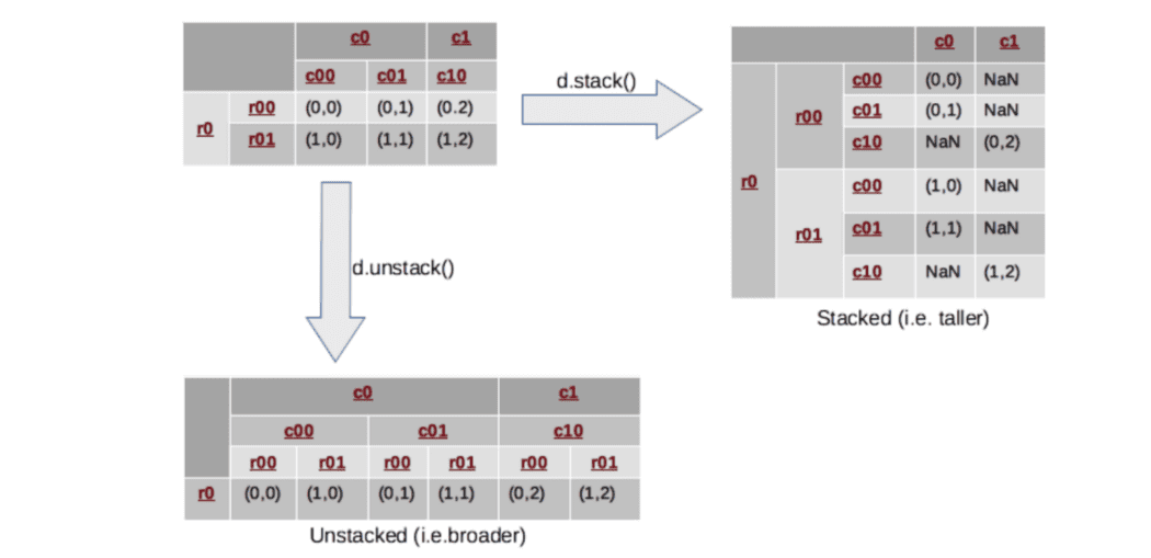
Therefore,
Stacking means rearranging the data vertically (or stacking it on top of each other, hence the name stacking), making the shape of the dataframe a taller and narrower stack (with fewer columns and more rows).
And unstacking will do just the opposite, spreading out the data and reshaping it into a shorter but wider dataframe (with fewer rows but more columns).